
Fibonacci sequence, among the ocean of integer sequences, has caught the attention of professional mathematicians and amateurs alike, for over centuries. While on the one side, it is a treasure house of numerous interesting mathematical properties, on the other side, the applications of Fibonacci sequence are widespread, including that of fractal music, financial market trading etc. Fibonacci numbers are found in many biological settings and nature, like the number of petals in sunflower, spiral phyllotaxis of plants and so on.
The elements of the Fibonacci sequence are generated by the second order recurrence relation
fn = fn-1 + fn-2
with the condition that f0=0,f1=1. It is also interesting to note that for a number x. to be a Fibonacci number, either 5x2+4 or 5x2−4 must be a a perfect square.
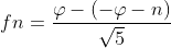
The ratio 
converges to the golden mean or the golden ratio 
The n-th Fibonacci number can be expressed in terms of the golden ratio as
In this work, we unfold yet another interesting result related to Fibonacci sequence from the perspective of discrete probability distributions generated by linear recurrence relations.
The classical Fibonacci sequence is known to exhibit many fascinating properties. In this paper, we explore the Fibonacci sequence and integer sequences generated by second order linear recurrence relations with positive integer coeffcients from the point of view of probability distributions that they induce. We obtain the generalizations of some of the known limiting properties of these probability distributions and present certain optimal properties of the classical Fibonacci sequence in this context. In addition, we also look at the self linear convolution of linear recurrence relations with positive integer coefficients. Analysis of self linear convolution is focused towards locating the maximum in the resulting sequence. This analysis, also highlights the influence that the largest positive real root, of the “characteristic equation” of the linear recurrence relations with positive integer coefficients, has on the location of the maximum. In particular, when the largest positive real root is 2, the location of the maximum is shown to depend on whether the sequence length being odd or even.
Key words: Fibonacci sequence, recurrence relations, probability distribution, limiting properties, linear convolution
AMS subject classifications. 11B37, 11B39, 60C05, 60C09, 60F99
Starting with any sequence  of positive real numbers, we can generate a probability distribution on {1;2;:::;N} for every N∈N as follows: Let X be a random variable taking values 1;2;:::;N such that
Starting with any sequence {f[n]}n∈N of positive real numbers, we can generate a probability distribution on {1;2;:::;N} for every N∈N as follows: Let X be a random variable taking values 1;2;:::;N such that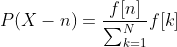
In particular, if f[n] are all positive integers, then we can generate such probability distributions using only integers. In a recent work, Neal [1] has investigated such probability distributions arising out of the Fibonacci sequence and obtained some limiting properties of these distributions as N→∞.
While exploring integer sequences from the point of view of generating window functions in the context of designing digital filters for signal processing applications [2], we found some generalizations of Neal’s limiting properties for a class of integer sequences and an optimal property of the Fibonacci sequence in this class. In this paper, we present these results.
The classical Fibonacci sequence [3], [4], is the positive integer sequence f[n] defined by the second order recurrence relation
f[n]=f[n−1]+f[n−2]
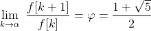
with initial conditions f[1]=1, f[2]=1. The ratio of successive terms of the Fibonacci sequence converges to the well known golden ratio φ, i.e.,
For any positive integer N, consider the Fibonacci sequence, f[1],f[2],…,f[N], of length N. Using the Fibonacci sequence, we can define a discrete probability distribution as follows. We define the probability mass function as1
pN [1], pN [2],….., pN [N]
pËN(n)=f[n]N∑k=1f[k]∀n=1,2,…,N
Let ËX be a random variable in {1,2,…,N} such that
P(ËX=n)=pËN(n);1≤n≤N.
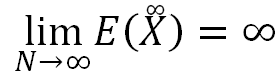
In his work, Neal [1] showed that, E(ËX), the mean or expectation of ËX, grows linearly as N increases and hence
limN→∞E(ËX)=∞
Similarly, let X_ be a random variable in {1,2,…,N}, where the probabilities, pN_[n], correspond to the Fibonacci sequence, of length N, in the decreasing order2. We define the probability mass function,
P(X_=n)=f[N+1−n]N∑k=1f[k]=pN_(n);1≤n≤N.
For such a random variable, X_, Neal [1] observed the following limiting properties:
limN→∞E(X_)=φ+1
limN→∞Var(X_)=2φ+1
where E(X_) denotes the mean or expectation of X_ and Var(X_) denotes the variance of X_.
The aim of this paper, as mentioned earlier, is to show that such limiting properties are characteristic for integer sequences defined by linear recurrence relations , of any order, with positive integer coefficients. For the sake of simplicity, we shall first discuss the second order recurrence relation.
Let a, b be any two positive integers and consider the integer sequence defined by the second order recurrence relation
f[n]=af[n−1]+bf[n−2]wheref[1]=1;f[2]=1;
The characteristic equation of this recurrence relation is given by
r2–ar–b=0.
It is well known that the solution to this Eq.(3.2) is given by
f[n]=C[R(a,b)n–Rs(a,b)n]
where,
R(a,b)=a+√a2+4b2
is the positive real root. The other root of the equation is
Rs=–bR(a,b)
and
C=1√a2+4b
We note that,
R(a,b)≥φforallpositiveintegersa,bR(a,b)=φwhena=b=1(classicalFibonaccisequence)
We further observe that the ratio of successive terms of this sequence converges to R(a,b), i.e.,
limk→∞f[k+1]f[k]=R(a,b)
As in section 2, for any positive integer N, consider the above sequence, of length N, i.e.,
f[1],f[2],…,f[N]
and define probability mass functions,
pËN(n)[1],pËN(n)[2],…,pËN(n)[N]
as
pËN(n)=f[n]N∑k=1f[k]∀n=1,2,…,N
Consider a random integer, ËX, in {1,2,…,N}, such that
P(ËX=n)=pËN(n)
Similarly let X_ be a random variable in {1,2,…,N}, (with probabilities corresponding to the decreasing sequence) such that,
P(X_=n)=f[N+1−n]N∑k=1f[k]=pN_(n)∀n=1,2,…,N
In the rest of the paper, for short, we shall denote R(a,b) by R and RS(a,b) by RS.
We prove the following limiting properties.
Analogous to eq.(2.5), we have,
Theorem 1.
Even though E(ËX) grows as N increases, its variance still converges. In fact, we have,
Theorem 2.
In the case of X_, both E(X_) and Var(X_) converge as N→∞ and the limit of Var(X_) is the same as that of Var(ËX). We have, analogous to eq.(2.7) and eq.(2.8), the following limits.
Theorem 3.
Theorem 4.
We, then, easily observe using these properties that when a=b=1, the limits of Theorem.(1), Theorem.(2) and Theorem.(3) reduce to the limits, eq.(2.5), eq.(2.7), eq.(2.8), obtained for the Fibonacci sequence, by Neal [1], described in section 2. Using eq.(3.3) and eq.(3.4), we can prove the following optimality properties of the Fibonacci sequence:
Theorem 5.
max(limN→∞E(X_):a,b∈N)=limN→∞(E(X_):a=b=1)=φ+1
Theorem 6.
max(limN→∞Var(ËX):a,b∈N)=max(limN→∞Var(X_):a,b∈N)=limN→∞(Var(X_):a=b=1)=2φ+1
We now proceed to prove these theorems.
In order to prove the aforesaid theorems, we make use of certain finite sums, presented in Appendix.A and Appendix.B. We list here, some of the notations used in the subsequent sections.
| Increasing sequence | Decreasing Sequence |
|---|---|
| ËS=N∑n=1f[n] | S_=N∑n=1f[N+1−n] |
| ËS1=N∑n=1nf[n] | S_1=N∑n=1nf[N+1−n] |
| ËS2=N∑n=1n2f[n] | S_2=N∑n=1n2f[N+1−n] |
We look at the mean and variance of the random variable ËX, defined as in section 2.
THEOREM 1:
limN→∞E(ËX)=∞
Proof :
We have,
E(ËX)=ËS1ËS
Using eq.(B.8) and eq.(B.6), we get
E(ËX)∼(NRN+2−(N+1)RN+1+R)(R−1)(R−1)2RN+1∼NR−N−1R−1⇒E(ËX)∼N–1R−1E(ËX)∼O(N)

Theorem 1, now follows from eq.(6.2).
We also observe the following:
If we now define ËY = (N+1)−ËX, so that ËY is also a random variable taking value 1, 2, 3, …, N and ËX has been in a sense centralized, then by eq.(6.2),
E(ËY)∼1+1R−1=RR−1
Hence
limN→∞E(ËY)=RR−1
This ËY corresponds to X_, which we describe in sec.7.
THEOREM 2:
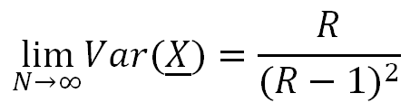
limN→∞Var(ËX)=R(R−1)2
Proof :
We have,
E(ËX2)=ËS2ËS
Using eq.(B.10) and eq.(B.6), we get
E(ËX2)∼N2(R−1)2–2N(R−1)+R+1(R−1)2
Using eq.(6.2) and eq.(6.4), we get
Var(ËX)=E(ËX2)−E(ËX)2∼N2(R−1)2–2N(R−1)+R+1(R−1)2−(N–1R−1)2⇒limN→∞Var(ËX)=(R+1)−1(R−1)2
Thus, we get the limit of the variance as,
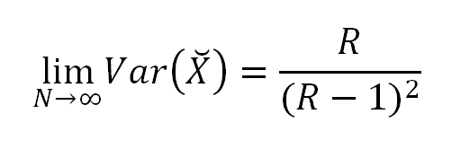
limN→∞Var(ËX)=R(R−1)2

It is interesting to note from eq.(6.2) and eq.(6.5) that, even though the mean increases linearly as the length of the sequence, the variance converges, to a function of R.
In this section, we look at the probability distribution generated by reversing the sequence values. We recall that the probability of the random variable X_ taking a value n was defined as,
P(X_=n)=f[N+1−n]N∑k=1f[N+1−k]=pN_(n)
THEOREM 3:
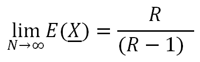
limN→∞E(X_)=1+1R−1=RR−1
Proof :
We have,
E(X_)=S_1S_
From eq.(B.13), we get
E(X_)=(N+1)ËS–ËS1ËS=(N+1)–ËS1ËS∼(N+1)–(N–1R−1)byeq.(6.2)⇒limN→∞E(X_)=1+1R−1=RR−1

THEOREM 4:
limN→∞E(X_2)=1+3R−1(R−1)2
Proof :
Var(X_)=E(X_2)–E(X_)2
Using eq.(B.14) we first obtain E(X_2).
E(X_2)=ËS2S_∼(N+1)2ËSËS–2(N+1)ËS1ËS+ËS2ËS∼(N+1)2–2(N+1)E(ËX)+E(ËX2)∼(N+1)2–2(N+1)(N−1R−1)+(N2(R−1)2–2N(R−1)+(R+1)(R−1)2)∼(R−1)2+3R−1(R−1)2
⇒limN→∞E(X_2)=1+3R−1(R−1)2
From eq.(7.3) and eq.(7.5), we get
Var(X_)=E(X_2)–E(X_)2→1+3R−1(R−1)2–R2(R−1)2⇒limN→∞Var(X_)=R(R−1)2

Thus, we find that, the limit of the variance of the probability distribution with probability defined by eq.(7.1) to be a simple function R, the limit of the ratio of successive elements.
Now, we look at the probability distribution induced by the standard Fibonacci sequence. For such a distribution, we obtain the value of mean and variance,using eq.(6.2) and eq.(7.5) respectively, by using a=1, b=1, and R=φ.
By eq.(6.2) and eq.(6.5), we have
E(ËX)∼O(N)
and
limN→∞Var(ËX)=R(R−1)2=φ(φ−1)2⇒limN→∞Var(ËX)=2φ+1
Neal [1] looks at the mean and variance of a Fibonacci distribution. It may be pointed out that the fact that the variance converges in this case was not observed by Neal. The above derivations show that, in this case, though the mean increases linearly as the length of the sequence, the variance converges to a simple function of the golden ratio φ.
By eq.(7.3), we have
limN→∞E(X_)=RR−1=φ+1
From eq.(7.6), we have
limN→∞Var(X_)=R(R−1)2=φ(φ−1)2⇒limN→∞Var(X_)=2φ+1
Comparing eq.(8.1) and eq.(8.2), we find that, in the case of the classical Fibonacci sequence, the variance of the distribution converges to the same value, irrespective of whether the probability values are increasing or decreasing.
In the following sections, we make a few observations and remarks related to the classical Fibonacci sequence.
We observe the curious fact that, from Theorem.(1) and Theorem.(2),
limN→∞Var(X_)E(X_)=1R−1
In the case a=b=1, that is, in the case of the distribution induced by the Fibonacci sequence, since R=φ
limN→∞Var(X_)E(X_)=1φ−1=φ
Thus the ratio of the variance of X_ to the expectation of X_ also converges to the Golden Ratio, φ.
In this section, we establish certain optimal probabilistic limit properties of the classical Fibonacci sequence.
THEOREM 5:
max(limN→∞E(X_):a,b∈N)=limN→∞(E(X_):a,b=1)=φ+1
Proof :
We know that
R≥φ⇒R−1≥φ−1⇒1R−1≤1φ−1
But φ = 1φ−1.
Hence, from eq.(10.1), we get
1R−1≤φ⇒1+1R−1≤1+φRR−1≤φ+1⇒limN→∞(E(X_):a,b∈N)≤limN→∞(E(X_):a=b=1)
Thus,
max(limN→∞E(X_):a,b∈N)=limN→∞(E(X_):a,b=1)=φ+1

Among the family of distributions, induced by second order linear recurrence relations with positive integer coefficients, a and b, the Fibonacci sequence gives the maximum limit for Var(X_), i.e.
THEOREM 6:
max(limN→∞Var(ËX):a,b∈N)=max(limN→∞Var(X_):a,b∈N)=limN→∞(Var(X_):a,b=1)=2φ+1
We prove this as follows:
Proof :
R≥φ⇒1R≤1φ⇒−1R≥–1φ⇒1−1R≥1–1φ⇒R(1−1R)2≥φ(1–1φ)2⇒1R(1−1R)2≤1φ(1–1φ)2
From eq.(10.6), we get
R(R−1)2≤φ(φ−1)2=2φ+1⇒R(R−1)2≤2φ+1⇒limN→∞(Var(X_):a,b∈N)≤limN→∞(Var(X_):a=b=1)

From eq.(10.8), we conclude that the limit variance of discrete probability distributions, induced by decreasing sequence and generated using second order linear recurrence, is maximum for the one generated using Fibonacci sequence.
In the next section, we consider the probability distributions generated by higher order recurrence relation with positive integer coefficients.
From Section.6 and Section.7, one can observe that the mean and variance of the probability distributions, induced by general second order linear recurrence relation with positive integer coefficients, depend only on the largest positive real root, R, of the associated “characteristic equation”. It turns out that, even in the case of any other higher order recurrence relation with positive integer coefficients, it is the largest positive real root that determines the mean and variance. We now proceed to prove the same. Let
f[n]=an−1f[n−1]+…+an−kf[n−k]∀ai∈N
be a kth order recurrence relation. The characteristic equation of this recurrence relation is given by,
f(x)=xk–an−1xk−1−…–an−k
Lemma 1.
Eq.(11.2), has atleast one real positive root and if α is the largest positive real root, then all the other roots (real and complex) lie within the disc |z|<α.
Using Lemma 1, it is easy to infer the following:
With R=α,
Thus, Theorem 5 can be generalized as
max(limN→∞E(X_):ai,i∈N)=limN→∞(E(X_):a1=a2=1,ai=0,∀i>2)=φ+1
and Theorem 6 can be further generalized as
max(limN→∞Var(ËX):ai,i∈N)=max(limN→∞Var(X_):ai,i∈N)=limN→∞(Var(X_):a1=a2=1,ai=0,∀i>2)=2φ+1
Now, we proceed to prove Lemma 1.
Proof :
By Descartes rule of signs, there exists a positive root. Since,
Let α be the largest positive root.
Claim: The root is simple.
Let f(x) be as in eq.(11.2). Since α is a root, we have
αk–an−1αk−1+…+an−k=0
Suppose, if α is a multiple root, then we must have
f′(α)=0
⇒kαk−1−(k−1)an−1αk−2+…+an−k+1=0
Multiplying by α, we get
kαk–(k−1)an−1αk−1+…+an−k+1α=0⇒kαk=(k−1)an−1αk−1+…+an−k+1α⇒<k(an−1αk−1+…+an−k+1α)⇒<k(an−1αk−1+…+an−k+1α+an−k)⇒αk<an−1αk−1+…+an−k+1α+an−k⇒αn<αn
This contradicts eq.(11.3). Hence α must be a simple root.
Now, we prove that all other roots of eq.(11.2) lie within the circle of radius α. Consider eq.(11.2), the characteristic equation of the corresponding kth order recurrence relation with positive integer coefficients. Since α is a root,
f(α)=0
Also, we have
limx→∞f(x)=∞⇒f(x)≥0,∀x≥αandf(x)>0∀x>α
Let β be any root (real or complex) of eq.(11.2). Clearly, β cannot be zero, because,
f(0)=−an−k<0
Let b = |β|.
Claim: b ≤ α
Reason: Suppose b > α.
Since β is a root, we have
f(β)=0⇒βk=an−1βk−1+…+an−kβn−k⇒|β|k=|an−1βk−1+…+an−kβn−k|⇒βk≤an−1|β|k−1+…+an−k|β|n−k
⇒βk−an−1|β|k−1–…–an−k|β|n−k≤0⇒bk−an−1bk−1–…–an−kbn−k≤0⇒f(b)≤0
However, since b > α, by eq.(11.7), f(b) > 0. Thus, we get a contradiction and hence b ≤ α.
Claim: b = α
Since β is a root, we have,
βk=an−1βk−1+…+an−kβn−k⇒|β|k=|an−1βk−1+…+an−kβn−k|
Since we have assumed that |β|=b=a,
αk=|an−1βk−1+…+an−kβn−k|
an−1αk−1+…+an−k=|an−1βk−1+…+an−k|byeq. (11.3)an−1|β|k−1+…+an−k=|an−1βk−1+…+an−k|
⇒an−1βk−1,…,an−k are all complex numbers in the same direction.
⇒an−k,an−k+1β are real positive
⇒β is real positive
⇒β=α.
Thus, based on the above claims, we find that
We prove that the largest positive real root of the characteristic equation, corresponding to higher order linear recurrence relation with integer coefficients, is greater than the golden ratio φ.
αk=an−1αk−1+…+an−kαn−k
Since all terms on the RHS are greater than 0
⇒αk>an−1αk−1+an−2αk−2⇒α2>an−1α+an−2
As an−1, an−2 are positive integers, we see that,
⇒α2>α+1⇒α2–α–1 >0
From the fact that, φ, the golden ratio, is the largest positive root of x2−x−1=0 and that x2−x−1>0 for x>φ, it follows that α is always greater than φ.

It must be noted that the distribution {pN_(n)},1≤n≤N, converges to a geometric distribution on N={1,2,3,…}. More precisely, we have the following:
Let Y be a random integer in N, such that
p(n)=P(Y=n)=ρn(1−ρρ)
where ρ=1R. We have,
∞∑n=1ρn=ρ1−ρ
and hence
∞∑n=1nρn−1=ddρ(ρ1−ρ)=1(1−ρ)2
Thus,
∞∑n=1nρn=ρ(1−ρ)2
Consequently,
E(Y)=∞∑n=1nρn(1−ρρ)=ρ(1−ρ)2(1−ρρ)=11−ρ=11−(1R)⇒E(Y)=RR−1
Similarly we can see that
Var(Y2)=R(R−1)2
Thus, we see that,
limN→∞E(X_)=E(Y)limN→∞Var(X_)=Var(Y)
We now show that the random variable X_ converges to the random variable Y in distribution.
We have for every n∈N,
pN_(n)∼(RN+1−nRN+1−R)(R−1)=(R−n1−R−N)(R−1)=(ρn1−ρN)(1ρ−1)=(ρn1−ρN)(1−ρρ)
Thus,
pN_(n)∼(ρn1−ρN)(1−ρρ)
Since limN→∞ρN=0 as ρ=1R<1, we have
limN→∞pN_(n)=ρn(1−ρρ)
From eq.(12.1) and eq.(12.5) we see that
limN→∞pN_(n)=p(n)∀n∈N
and thus X_ converges to Y in distribution.
In the previous subsection, we observed that the distributions generated by second order linear recurrence relation converge to a geometric distribution, i.e.,
Now, we prove that all the moments of X_ converge to the corresponding moment of Y, as N→∞.
Proof :
For any positive integer k, we have,
E(X_k)∼N∑n=1nkRN+1−nN∑n=1RN+1−n
We have,
N∑n=1RN+1−n=RN+1−RR−1
Also,
N∑n=1nkRN+1−n=RN+1N∑n=1nkR−n
Substituting eq.(13.2) and eq.(13.3) in eq.(13.1), we get
E(X_k)∼(RN+1N∑n=1nkR−nRN+1−R)(R−1)=(RN+1N∑n=1nkR−nRN+1(1−R−N))(R−1)=N∑n=1nkρn1−R−N(1−ρρ)
Hence, as N→∞,
E(X_k)â¶N∑n=1nkρn(1−ρρ)becauseR−N→0=E(Yk)
Thus, we have for every non-negative integer k,
showing that all the moments of X_ converge to the corresponding moments of Y.

The moments of the probability distribution induced by classical Fibonacci sequence converge to a linear function of the Golden ratio, φ.
Proof :
We have,
∞∑n=1xn=x1−xfor|x|<1.
which on differentiation gives
∞∑n=1nxn−1=1(1−x)2
From eq.(13.4), we get
∞∑n=1nxn=x(1−x)2
Then,
∞∑n=1nxn(1−xx)=1(1−x)
Similarly, differentiating eq.(13.5), we get
∞∑n=1n2xn−1=(1−x)2+2x(1−x)(1−x)4=(1−x)+2x(1−x)3=1+x(1−x)3
and hence,
∞∑n=1n2xn=(1+x)x(1−x)3
and thus,
∞∑n=1n2xn(1−xx)=1+x(1−x)2
We shall now show, by induction, that in general, for any positive integer k,
∞∑n=1nkxn(1−xx)=Pk−1(x)(1−x)k
where Pk−1(x) is a polynomial in x of degree k−1.
We have from eq.(13.6) and eq.(13.7), that the result eq.(13.9) is true for k=1 and k=2. Thus, it is enough to show that if eq.(13.9) is true for some k=r, then it is also true for k=r+1. Suppose eq.(13.9) is true for k=r, then
∞∑n=1nrxn(1−xx)=Pr−1(x)(1−x)r
Hence, we get,
∞∑n=1nrxn=xPr−1(x)(1−x)r
On differentiating eq.(13.10), we get,
∞∑n=1nr+1xn−1=(1−x)r+1{Pr−1(x)+P′r−1(x)}+xPr−1(x)r(1−x)r(1−x)2r+2=(1−x){Pr−1(x)+xP′r−1(x)}+xPr−1(x)r(1−x)r+2=Pr(x)(1−x)r+2
where
Pr(x)=(1−x){Pr−1(x)+xP′r−1(x)}+xPr−1(x)r
is a polynomial of degree r. From eq.(13.11), we get,
∞∑n=1nr+1xn=xPr(x)(1−x)r+2
and hence,
∞∑n=1nr+1xn(1−xx)=Pr(x)(1−x)r+1
and thus proving that if eq.(13.9) is true for k=r, then it is also true for k=r+1. Thus by induction, we get eq.(13.9) is true for all k.
From eq.(13.9), we get
E(Yk)=∞∑n=1nkρn(1−ρρ)=Pk−1(ρ)(1−ρ)k
and hence
limN→∞E(X_k)=E(Yk)=Pk−1(ρ)(1−ρ)k
eq.(13.13) is a rational function of ρ and hence a rational function of R. In particular, for the classical Fibonacci sequence, we have
limN→∞E(X_k)=E(Yk)=Pk−1(1φ)(1−1φ)k
Since 1φ=φ−1, we get
limN→∞E(X_k)=E(Yk)=(Pk−1(φ−1)(φ−1)k)φk=φ2kPk−1(φ−1)=Q(φ),apolynomialinφ
But, since φ2=φ+1, all powers φj for j≥2 can be expressed as linear polynomials in φ and hence we get any polynomial in φ can be rewritten as a linear polynomial in φ. Thus,
limN→∞E(X_k)=E(Y)=Akφ+Bk

We now provide a detailed analysis about the location of the maximum in the sequence resulting from self linear convolution of linear recurrence relations with positive integer sequences.
In the previous sections, we proved certain optimal properties of the classical Fibonacci sequence among the general k-th order recurrence relations with positive integer coefficients, with respect to the discrete probability distributions that they induced. In this section we bring out another fascinating property of the classical Fibonacci sequence. Let xn be a finite length integer sequence, of length N, generated by a k-th order recurrence relation with positive integer coefficients. The location of maxima in the sequence, yn resulting from the linear convolution of xn with itself, can be only one of the following:
We prove the above in the following sections.
As mentioned earlier, while investigating the use of integer sequences for window functions in digital filtering [2], we observed that most of the integer sequences generated by k-th order recurrence relations, with positive integer coefficients, are non-decreasing. However, conventional classical window functions are symmetric, bounded and smooth. Though, integer sequences, mentioned as above, are bounded for finite length, they are not symmetric. Hence to be used as window functions, integer sequences are symmetrized. However, this does not guarantee a smooth profile for most of the integer sequences. In order to get a smooth profile, we do one of the following:
While in the first case, for any finite length, N, one can symmetrize at half the length, the second case requires the location of maximum in the sequence resulting from the linear convolution. In the sections to follow, we obtain the location of maxima in the sequence resulting from the linear convolution of xn with itself. In particular, we look at the family of sequences generated using k-th order linear recurrence relation. First, we look at the second order case and then generalize the result to higher order recurrence relations.
Let
x={xn}Nn=1y={yn}2Nn=2xn=axn−1+bxn−2,∀a,b∈N
The “characteristic” equation of the above is given by
x2–ax–b=0
The largest positive real root of the above equation is as below:
R=a+√a2+4b2
The linear convolution of two sequences is given by
yn=n−1∑k=1xkxn−k2≤n≤NyN+j=N∑k=jxkxN+j−k1≤j≤N
For 2≤n≤N, we have,
yn–yn−1=n−1∑k=1xkxn−k–n−2∑k=1xkxn−1−k=n−2∑k=1xk(xn−k−xn−1−k)+xn−1x1>0⇒yn>yn−11≤n≤N
From eq.(15.10), we observe that the convolution sum is an increasing sequence for 1≤n≤N.
Now we look at the eq.15.7, for j≥1.
yN+j–yN+j−1=N∑k=jxkxN+j−k–N∑k=j−1xkxN+j−1−k
At this juncture, we revisit the general second order recurrence relation with positive integer coefficients, given in eq.(15.3). We evaluate eq.(15.3) for different possible values of a and b and hence compute the difference as in eq.(15.11).
We look at case(Ai) that corresponds to a=b=1. Eq.(15.3), in this case, generates the elements of classical Fibonacci sequence. Eq.(15.3) can be rewritten as
xn=xn−1+xn−2
R, the largest positive real root in the case of classical Fibonacci sequence corresponds to the golden ratio, φ=(1+√52),
With the above conditions, eq.15.11 gives
yN+j–yN+j−1=N∑k=jxkxN+j−k–N∑k=j−1xkxN+j−1−k=N∑k=jxk(xN+j−1−k+xN+j−2−k)–N∑k=j−1xkxN+j−1−k=N∑k=jxkxN+j−2−k–xj−1xN
Suppose, j≤N−1,
yN+j–yN+j−1≥xN−1xj−1+xNxj−2–xj−1xN=xN−1xj−1+xN(xj−1−xj−3)−xj−1xN=xN−1xj−1–xj−3xN=xN−1(xj−2+xj−3)–xj−3(xN−1+xN−2)Rearrangingtheterms,weget=xN−1(xj−2–xj−3)+xj−3(xN−1–xN−2)
We find that the term on the right hand side, in the above equation is greater than 0. Hence
yN+j–yN+j−1>0
From eq.(16.3), we find the sequence yn to be increasing for 1≤j≤N−1. The only pair of elements of yn that needs to be compared are y2N and y2N−1. From eq.(16.2), we get For N−1≤j≤N, the above corresponds to
y2N–y2N−1=x2N–2xNxN−1=xN(xN–2xN−1)=xN(xN−2−xN−1)sincexN=xN−1+xN−2
We know that xn<xn+1, and hence, from the above equation, we have
⇒y2N–y2N−1<0
From eq.(16.5), we find that y2N<y2N−1. Thus, in the sequence resulting from the linear convolution of finite length classical Fibonacci sequence with itself, the maximum is located at 2N−1, where N is the length of the sequence xn.
Now, we explore what happens when a=1,b=2 in eq.(15.3), as mentioned in case(Aii). The corresponding second order recurrence relation is as below:
xn=xn−1+2xn−2
In this case, the “characteristic” equation is x2–x–2=0 and the largest positive root, R, is 2. To obtain the location of the maximum in the linear convolution of eq.17.1 with itself, we adopt the same procedure as classical Fibonacci sequence.
yN+j–yN+j−1=N∑k=jxkxN+j−k–N∑k=j−1xkxN+j−1−k=N∑k=jxk(xN+j−1−k+2xN+j−2−k)–N∑k=j−1xkxN+j−1−k=N∑k=j2xkxN+j−2−k−xj−1xN
Suppose, j≤N−1,
yN+j–yN+j−1≥2xN−1xj−1+xNxj−2–xj−1xN≥2xN−1xj−1+xN(xj−1−2xj−3)−xj−1xN=2xN−1xj−1–2xj−3xN=2xN−1(xj−2+2xj−3)–2xj−3(xN−1+2xN−2)
Rearranging the terms, we get,
=2xN−1(xj−2–2xj−3)+4xj−3(xN−1–xN−2)yN+j–yN+j−1>0
From eq.(17.4), we find the sequence yn to be an increasing one for 1≤j≤N−1. The only elements of yn that need to be compared are y2N and y2N−1. For N−1≤j≤N, the above corresponds to
y2N–y2N−1=x2N–2xNxN−1=xN(xN–2xN−1)
This can be easily proved by mathematical induction.
Proof :
Let k = 2. With standard initial conditions 1, 1 one can observe that f2<12f3 and f2<2f1.
Let k = 4. The sequence elements with initial conditions 1, 1 turn out to be 1, 1, 3, 5. We observe that f4<12f5 and f4<2f3.
For any k, we prove the following by induction.
f2k<min{2f2k−1,12f2k+1}
Let eq.(17.7) be true for k-1. So, we have
f2k−2<min{2f2k−3,12f2k−1}
We now prove that eq.(17.7) is true for k i.e.,
f2k<min{2f2k−1,12f2k+1}
f2k=f2k−1+2f2k−2
We know that from eq.(17.8), f2k−2<12f2k−1
Hencef2k<f2k−1+f2k−1⇒f2k<2f2k−1
Similarly,
f2k+1=f2k+2f2k−1
From eq.(17.10), f2k<2f2k−1
Hencef2k<f2k+1−f2k⇒2f2k<f2k+1⇒f2k<12f2k+1
Thus we find that, f2k<min{2f2k−1,12f2k+1}. From this one can see that yn has its maximum either at 2N-1 or 2N depending on whether the sequence length is odd or even.

With a=1,b>2 in eq.(15.3), we look at case(Aiii). The corresponding second order recurrence relation is as below:
xn=xn−1+bxn−2
In this case, the “characteristic” equation is x2–x–b=0 and the largest positive root, R, greater than 2. We now proceed to obtain the location of the maximum in the linear convolution of eq.(18.1) with itself.
yN+j–yN+j−1=N∑k=jxkxN+j−k–N∑k=j−1xkxN+j−1−k=N∑k=jxk(xN+j−1−k+bxN+j−2−k)–N∑k=j−1xkxN+j−1−k=N∑k=jbxkxN+j−2−k−xj−1xN
Suppose, j≤N−1,
yN+j–yN+j−1≥bxN−1xj−1+bxNxj−2–xj−1xN≥bxN−1xj−1+bxN(xj−1−bxj−3)−xj−1xN=bxN−1xj−1–bxj−3xN=bxN−1(xj−2+bxj−3)–bxj−3(xN−1+bxN−2)
Rearranging the terms, we get,
=bxN−1(xj−2–xj−3)+b2xj−3(xN−1–xN−2)yN+j–yN+j−1>0
From eq.(18.4), we find the sequence yn to be an increasing one for 1≤j≤N−1. The only elements of yn that need to be compared are y2N and y2N−1.
For N−1≤j≤N, the above corresponds to
y2N–y2N−1=x2N–2xNxN−1=xN(xN–2xN−1)=xN(xN−1+bxN−2−2xN−1)
Let us consider the sequence generated by eq.(18.1), with b=3. The elements of the sequence, with initial values being 1, 1, are
From the above, we find that bxn−2 is always greater than xn−1. Thus eq.18.7 is always positive. Hence, we find that y2N>y2N−1. Thus, the maximum is located at 2N and not at 2N−1. A formal proof by induction can be obtained along the same lines of mathematical induction, as found in section.17.
a>1:
We now present the case when a>1 and b∈N, in eq.(15.3).
yN+j–yN+j−1=N∑k=jxkxN+j−k–N∑k=j−1xkxN+j−1−k=N∑k=jxk(axN+j−1−k+bxN+j−2−k)–N∑k=j−1xkxN+j−1−k=N∑k=j(a−1)xkxN+j−1−k+N∑k=jbxkxN+j−2−k−xj−1xN
When a>1, the term xj−1xN gets accounted for by N∑k=j(a−1)xkxN+j−1−k, with k=N. The remaining terms are all positive. Hence yn increases till 2N−1. Now, we compare y2N−1 and y2N.
For N−1≤j≤N, the above corresponds to
y2N–y2N−1=x2N–2xNxN−1=xN(xN–2xN−1)=xN(axN−1+bxN−2−2xN−1)=xN((a−2)xN−1+bxN−2)
With a>1 and b∈N, eq.(18.13) is always positive. Hence y(n) has its maximum at y2N.
In the previous section, we found that the sequence resulting from the self linear convolution of second order linear recurrence (with positive integer coefficients) has its maximum located at either 2N-1 or 2N is determined by the
It was proved that, when the largest positive real root was 2, the location of maximum is either 2N-1 or 2N, based on whether N, the length of xn, is even or odd.
It is also worth noting that this is true even in the case of self convolution of, xn=axn−1, first order linear recurrence relation (with positive integer coefficients). In this case, if a = 2, the largest positive real root is 2. yn has its maximum at either 2N-1 or 2N depending on whether the length N is even or odd. However, when a = 1, it can be easily proved that, the maximum of yn is located at N.
Now, we look at the higher order recurrence relations with positive integer coefficients. Let
xn=an−1xn−1+…+akxn−k∀ai∈N
be a higher order recurrence relation. On similar lines, as self linear convolution of the second order linear recurrence relation, one can establish that even in the case of higher order recurrence relations, there exist three cases, namely,
In this work, on the one hand, we have explored and proved certain optimal probabilistic limit properties of Fibonacci sequence. We have proved that, among the distributions induced by kth order linear recurrence equations with positive integer coefficients, the limits of the mean and the variance are maximum for those generated by second order linear recurrence relation, corresponding to the Fibonacci sequence. We also found that the ratio of the variance to the mean, of the distribution induced by the Fibonacci sequence turns out to be golden ratio, φ. Moreover, for all such distributions, we have,
Besides proving certain optimal probabilistic limit properties, we also analyzed the second order linear recurrence relation with positive integer coefficients, from the point of view of self linear convolution. We established that the sequence resulting from the self linear convolution of any higher order linear recurrence relation with integer coefficients, can have its maximum either at 2N or 2N-1. A more interesting observation in this regard is that when the largest positive real root of such recurrence relations is 2, the location of maximum depends on whether the sequence length of xn is odd or even.
Appendix A.
Some Preliminaries.
We list some of the identities used in this paper in the following sections.
G(x)=N∑n=1xn=x+x2+…+xN=xN+1−xx−1
Let G′(x) be the derivative of G(x). We have,
G′(x)=1+2x+…+NxN−1=(x−1){(N+1)xN−1}−(xN+1−x)(x−1)2=(N+1)xN+1−x−(N+1)xN+1−xN+1+x(x−1)2=NxN+1−(N+1)xN+1(x−1)2
Hence, we get,
xG′(x)=N∑n=1nxn=x+2x2+…+NxN=NxN+2−(N+1)xN+1+x(x−1)2
From this we get,
(xG′(x))′=1+22x+…+N2xN−1
which by eq.(A.2) is
(xG′(x))′=(x−1)2{N(N+2)xN+1−(N+1)2xN+1}−2(x−1){NxN+2−(N+1)xN+1+x}(x−1)4=(x−1){N(N+2)xN+1−(N+1)2xN+1}−2{NxN+2−(N+1)xN+1+x}(x−1)3=N2{xN+2−2xN+1+xN}+N{−2xN+1+2xN}+{xN+1+xN+x+1}(x−1)3
and hence,
x(xG′(x))′=N∑n=1n2xn=N2{xN+3−2xN+2+xN+1}+N{−2xN+2+2xN+1}+{xN+2+xN+1+x2+x}(x−1)3
Appendix B.
Useful Finite Sums.
In this section, we obtain the expressions for some of the finite sums relevant to the work presented in this paper.
B.1. N∑n=1f[n]
Let ËS be the sum of the sequence f[n] defined as
ËS=N∑n=1f[n]=N∑n=11√a2+4b(Rn–RnS)
From eq.(A.1), we get
G(R)=R+R2+R3+…+RN=N∑n=1Rn=RN+1−RR−1
G(RS)=RS+R2S+R3S+…+RNS=N∑n=1RnS=RN+1S−RSRS−1
Substituting eq.(B.2) and eq.(B.3) eq.(B.1), we get,
ËS=1√a2+4bN∑n=1(G(R)–G(RS))=1√a2+4b(RN+1−RR−1–RN+1S−RSRS−1)
We have,
R2=2a2+4b+2a√a2+4b4⇒R2>b⇒|RSR|=bR2<1
Hence, taking RN+1 common from eq.(B.4), we see that,
ËS∼1√a2+4b(RN+1R−1)
B.2. N∑n=1nf[n]
Let ËS1 be defined as
ËS1=N∑n=1nf[n]
ËS1=N∑n=1nf[n]=1√a2+4bN∑n=1(nRn–n(RS)n)
By eq.(A.2), we get
N∑n=1nRn=NRN+2−(N+1)RN+1+R(R−1)2
We can get a similar expression involving the other root RS. Using the fact that the absolute value of the ratio of RS and R is less than 1, we obtain
ËS1∼1√a2+4b(NRN+2−(N+1)RN+1+R(R−1)2)
B.3. N∑n=1n2f[n].
Let ËS2 be defined as
ËS2=N∑n=1n2f[n]
Using eq.(A.4) we get
ËS2∼N2{RN+3−2RN+2+RN+1}+N{−2RN+2+2RN+1}+{RN+2+RN+1+R2+R}(R−1)3
B.4. N∑n=1f[N+1−n].
Let S_ be defined as
S_=N∑n=1f[N+1−n]Clearly,ËS=N∑n=1f[n]=N∑n=1f[N+1−n]=S_
Thus the sum S_ = ËS , where ËS is as in eq.(B.6).
B.5. N∑n=1nf[N+1−n].
Let S_1 denote N∑n=1nf[N+1−n]
S_1=N∑n=1nf[N+1−n]=−N∑n=1(−n)f[N+1−n]=–N∑n=1(N+1−n)f[N+1−n]+(N+1)N∑n=1f[N+1−n]=–N∑k=1kf[k]+(N+1)ËS⇒S_1=(N+1)ËS–ËS1
B.6. N∑n=1n2f[N+1−n].
Let S_2 be defined as
S_2=N∑n=1n2f[N+1−n]=N∑n=1(N+1−n)2f[n]=(N+1)2N∑n=1f[n]–2(N+1)N∑n=1nf[n]+N∑n=1n2f[n]⇒S_2=(N+1)2ËS−2(N+1)ËS1+ËS2
where ËS1 and ËS2 are as in eq.(B.7) and in eq.(B.9) respectively.
[1] D. K. Neal, Limits of Mean and Variance of a Fibonacci Distribution, Math. Scientist 34, 2009, pp. 25-29.
[2] Arulalan Rajan, Some applications of Integer sequences in signal processing and their implications on performance and architecture, PhD thesis, Indian Institute of Science, September 2011.
[3] N. J. A. Sloane, The On-Line Encyclopedia of Integer Sequences, Ed.2008, published electronically at
[4] S. Vajda, Fibonacci and Lucas Numbers, and the Golden Section: Theory and Applications, Dover, 2008.