
Recursion is a powerful concept that can yield succinct algorithms for solving complex computational problems, using the divide-and-conquer paradigm (or its special case: decrease-and-conquer). Succinct algorithms tend to be easy to implement and read, and hence the ability to create recursive algorithms and the ability to read and write recursive code are key skills for any programmer. Students often find recursion a challenging concept to understand, and several researchers have investigated the causes for these challenges and possible solutions. We recommend the following surveys as an introduction to this body of research [6], [7], [8], and we discuss some of the key challenges below.
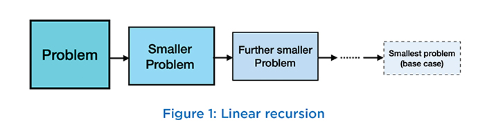
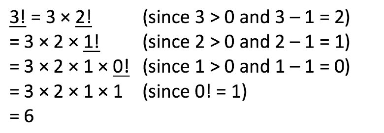
Any recursive algorithm solves a “large” problem by decomposing it into one or more “smaller” problems, and then combining the solution(s) to these smaller problem(s) into a solution to the original problem. The recursion stops when the problem cannot be decomposed further, and this is called a base case of the recursion. The simplest Given an inductive definition such as Equation 1, consider the following steps for calculating ![]() In each step, the underlined value is substituted according to Equation 1. form of recursion is linear, where the large problem is broken into a single smaller problem as shown in Figure 1, leading to decrease-and-conquer algorithms. (There must always be at least one base case, but there can be several base cases, even with linear recursion.)
In each step, the underlined value is substituted according to Equation 1. form of recursion is linear, where the large problem is broken into a single smaller problem as shown in Figure 1, leading to decrease-and-conquer algorithms. (There must always be at least one base case, but there can be several base cases, even with linear recursion.)
A typical example of linear recursion is the recursively defined factorial function for non-negative integers: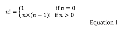
Here, the “large” problem is to calculate the factorial of ![]() and this problem is decomposed into a single “smaller” problem, which is to calculate the factorial of
and this problem is decomposed into a single “smaller” problem, which is to calculate the factorial of ![]() Finally, the solution to this sub-problem must be multiplied with
Finally, the solution to this sub-problem must be multiplied with ![]() to calculate the solution to the original problem (the factorial of
to calculate the solution to the original problem (the factorial of ![]() ). Here, there is a single base case for
). Here, there is a single base case for ![]() Students are usually at least somewhat familiar with such inductive definitions on integers, and are able to at least read the recursive implementation corresponding to this definition:
Students are usually at least somewhat familiar with such inductive definitions on integers, and are able to at least read the recursive implementation corresponding to this definition: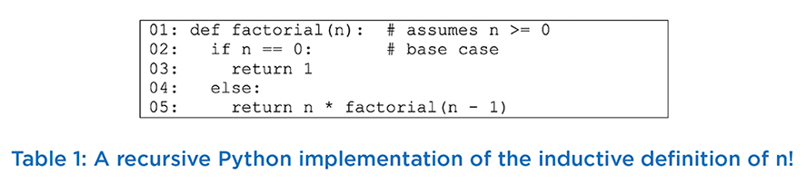
Tunnel Wilson et al. [9] hypothesize that this “substitution model offers students a mechanical, consistent, and simple way of tracing recursion”. In our experience as well, most students can correctly perform such steps. In contrast, we find that students start struggling when asked to trace the step-by-step execution of the corresponding code (Table1). One reason for this struggle is because students must keep track of the stack of recursive calls and the pending “work” that must be done to “combine” the result of each recursive call to produce the solution. Note that this work is much easier to represent in the substitution model: it is precisely the part of each line in the derivation above that is not underlined, and students can keep track of it in each line simply by copying it from the previous line.
Another important reason why students struggle to trace recursive code is because they must distinguish between multiple copies of the recursive function’s arguments (![]() in this case), all of which have the same name but potentially hold different values, and they must keep track of each recursive call’s return value. All these values are held in the call stack, as shown in Figure 2.
in this case), all of which have the same name but potentially hold different values, and they must keep track of each recursive call’s return value. All these values are held in the call stack, as shown in Figure 2.
When students are first exposed to recursion, they find it hard to visualize how recursion works using the same code repeatedly. They are typically just becoming familiar with how the call stack works, and it is easy for them to make mistakes, especially how does same variable take different value with each call stack invocation and return. In contrast, students may be far more comfortable with an iterative algorithm for computing n! that uses a simple loop to compute the product 1 × 2 × … × n, and they may fail to see the power of the decrease-and-conquer approach. Thus, it becomes important to expose students to problems where iterative solutions are non-obvious whereas simple recursive solutions exist. Such problems typically require non-linear recursion, where the “large” problem must be decomposed into more than one subproblem (the “divide” step), and the recursively computed solutions to these sub-problems must be combined into a solution to the original problem (the “conquer” step). Such problems, which include recursive algorithms for binary trees and the well-known “Tower of Hanoi” problem, tend to be even more challenging for students to trace. Although the latter problem deals with familiar integers, many students are unable to trace the algorithm accurately. The first author conducted the following exercise: A class size of just over 60 students was divided into 15 groups (each group with at least 4 members). Each group was asked to demonstrate algorithm for the Tower of Hanoi problem,which they had studied in an earlier semester, with 5 discs. After 20 minutes, only one group was able to demonstrate the optimal sequence of 31 moves. Hence it is important to introduce at least one effective example of linear recursion as early as possible. We will discuss such an example in the
next section.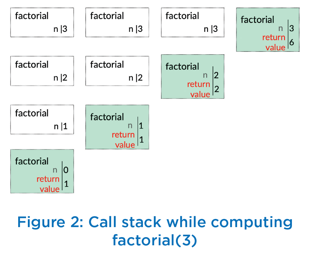
Apart from the challenge of tracing recursive code, two other key challenges for students are to formulate recursive algorithms to solve problems, and to accurately implement these algorithms. We will defer our discussion of this challenges to the next article.
In line with our Gamified Approach to Learning Algorithms (GALA) [1], let us motivate the power of (linear) recursion with the following puzzle. Suppose you are Person ![]() standing in a queue at an airport check-in counter, as shown in Figure 3. You cannot see the end of queue, but you would like to determine your position in the queue to estimate the waiting time before your turn. If the queue is modeled as a list of people, students will find it easy to propose a simple iterative solution that calculates the length of the list. Such an algorithm evokes a mental image of “walking along the queue” from your position to the end and counting the number of people. To prevent students from thinking along these lines, we inform students that their algorithm can only check if there is someone ahead of them in the queue and, if so, they can ask that person a question and use that answer to determine the queue length. What would be the approach you would like to take to determine your position in the queue? Consider this before reading ahead. Here is a simple recursive algorithm: If there is no one ahead of you, then clearly your position in the queue is 1 (the base case). Otherwise, ask the person in front of you: What is your position in the queue? (That person will compute the answer recursively!) Finally, add one to that person’s answer.
standing in a queue at an airport check-in counter, as shown in Figure 3. You cannot see the end of queue, but you would like to determine your position in the queue to estimate the waiting time before your turn. If the queue is modeled as a list of people, students will find it easy to propose a simple iterative solution that calculates the length of the list. Such an algorithm evokes a mental image of “walking along the queue” from your position to the end and counting the number of people. To prevent students from thinking along these lines, we inform students that their algorithm can only check if there is someone ahead of them in the queue and, if so, they can ask that person a question and use that answer to determine the queue length. What would be the approach you would like to take to determine your position in the queue? Consider this before reading ahead. Here is a simple recursive algorithm: If there is no one ahead of you, then clearly your position in the queue is 1 (the base case). Otherwise, ask the person in front of you: What is your position in the queue? (That person will compute the answer recursively!) Finally, add one to that person’s answer.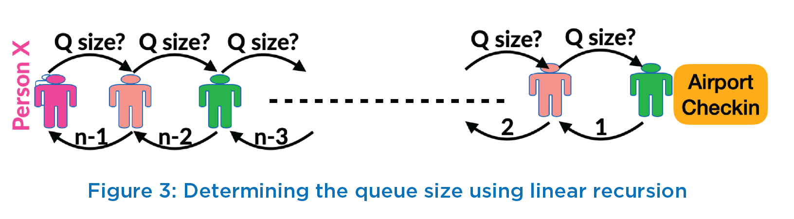
When we present this puzzle in class, many students are able to articulate the key idea of adding one to the previous person’s position. However, they struggle to express their thinking clearly in recursive form (as above). Instead, here is a typical student articulation:
Ask the person ahead of you about queue size for them. That person also does not know the queue size, so he/she must ask the next person ahead of him/ her. The process repeats till the question is asked to the first person (the person at the counter). Since the queue ends at this person, this person responds with queue size of 1. The second person adds 1 to it and responds back to the third person with queue size of 2. Thus, each person adds 1 to the queue size value received from the person ahead and responds to the person behind with the updated value of queue size. Finally, you (person X) get some value ![]() – 1 from the person ahead of you, and you add 1 to determine the queue size to be
– 1 from the person ahead of you, and you add 1 to determine the queue size to be ![]() .
.
Notice how this articulation is much longer. Further, it describes the execution of the recursive algorithm rather than the algorithm itself. We point out this distinction and request students to refine their articulation. In particular, they are not allowed to use expressions such as “…repeat this until…”, “…and so on…”, etc. When students finally arrive at a crisp recursive formulation, some of them begin to appreciate the beauty and power of recursion. On the other hand, some students remain uncomfortable with the seemingly mysterious way in which the computation steps are hidden within the recursive function call. To dispel this mystery, we show students an implementation of the recursive algorithm (Table 2) and trace through the code. Here, the function next(x) returns the person ahead of x in the queue (or None, if x is the first person in the queue).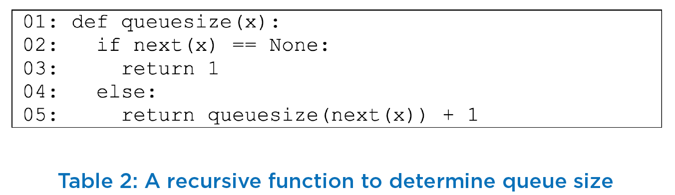
Puzzle 2: Neumann’s neighbourhood
The purpose of our next puzzle is to introduce students to the idea of recurrence relations, initially in the simplified
setting of linear recursion. Consider the Neumann’s neighbourhood problem (as discussed in [6]), which is to determine
the total number of one-by-one squares T(![]() ) after n stages of the process shown Figure 5 [3][4].
) after n stages of the process shown Figure 5 [3][4].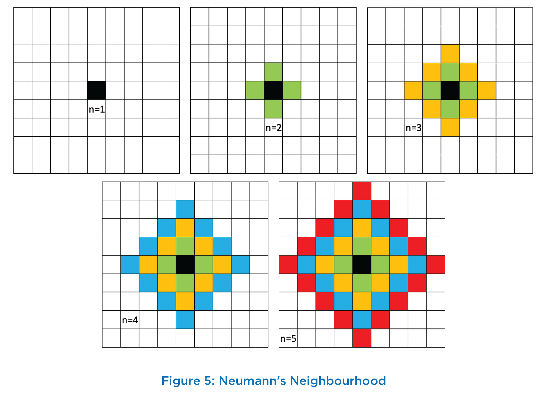
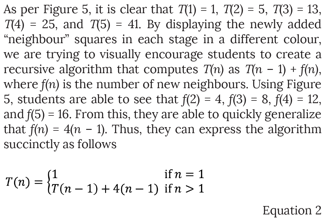
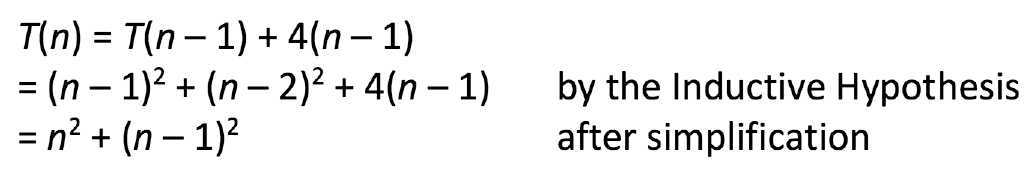
This is an example of a recurrence relation, which students will later see in the context of analyzing the complexity of recursive algorithms. We therefore include a short discussion on how recurrence relations can be solved. In this case, there is a neat closed-form solution that can easily be verified by mathematical induction: ![]()
![]() The base case of the induction
The base case of the induction ![]() clearly holds. Further, for any
clearly holds. Further, for any ![]()
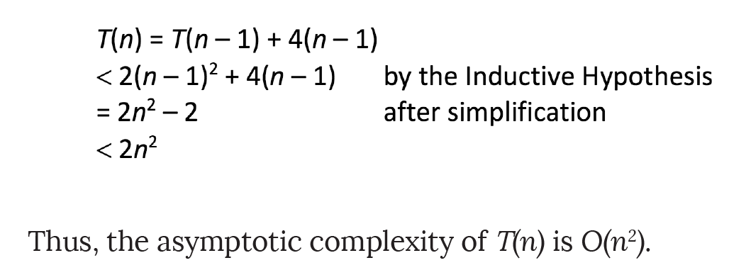
For some recurrence relations that students will encounter later, it may not be easy to derive an exact closed-form solution. Often, an upper-bound on ![]() is sufficient (e.g., for computing the algorithm’s worst-case complexity). In this case, a similar inductive proof can show that
is sufficient (e.g., for computing the algorithm’s worst-case complexity). In this case, a similar inductive proof can show that ![]() Many students are far less comfortable with manipulating inequalities, so we show the full proof. The base case of the induction
Many students are far less comfortable with manipulating inequalities, so we show the full proof. The base case of the induction ![]() clearly holds. Further, for any
clearly holds. Further, for any ![]()
Another interesting puzzle involving recursion is to solve the problem of alternating discs [5]. Suppose there are ![]() discs of two alternating colors black and red (Figure 6). Students are asked to rearrange these discs such that all red discs appear before all black discs, but the only move When
discs of two alternating colors black and red (Figure 6). Students are asked to rearrange these discs such that all red discs appear before all black discs, but the only move When ![]() = 1 (i.e., 2 discs), clearly only one swap is needed, as shown in Figure 7(a). Now consider the case when n > 1. Clearly, any algorithm would have to swap the first (leftmost) black disc with each of the
= 1 (i.e., 2 discs), clearly only one swap is needed, as shown in Figure 7(a). Now consider the case when n > 1. Clearly, any algorithm would have to swap the first (leftmost) black disc with each of the ![]() red discs to its right one at a time. This would require at least n swaps. Similarly, the algorithm would have to swap the second black disc with each of the
red discs to its right one at a time. This would require at least n swaps. Similarly, the algorithm would have to swap the second black disc with each of the ![]() – 1 red discs to its right. (It need not swap it with the red disc to its left, because that allowed is interchange (swap) of two neighbouring discs. The problem is to count the minimum number of swaps required to achieve this rearrangement. Before proceeding to discuss the solution, we recommend that you pause and work it out.
– 1 red discs to its right. (It need not swap it with the red disc to its left, because that allowed is interchange (swap) of two neighbouring discs. The problem is to count the minimum number of swaps required to achieve this rearrangement. Before proceeding to discuss the solution, we recommend that you pause and work it out.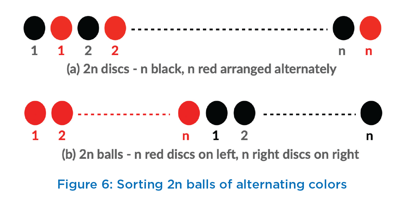
would be unnecessary.) Thus, the minimum number of swaps so far is ![]() +
+ ![]() – 1. Continuing like this, we can argue that the algorithm would have to swap the last (rightmost) black disc with 1 red disc. Hence, the minimum number of swaps in total is
– 1. Continuing like this, we can argue that the algorithm would have to swap the last (rightmost) black disc with 1 red disc. Hence, the minimum number of swaps in total is ![]() +
+ ![]() – 1 + … + 1, which is
– 1 + … + 1, which is ![]() (
(![]() + 1)/2. This argument can be made more precise using induction, but we omit this here.
+ 1)/2. This argument can be made more precise using induction, but we omit this here.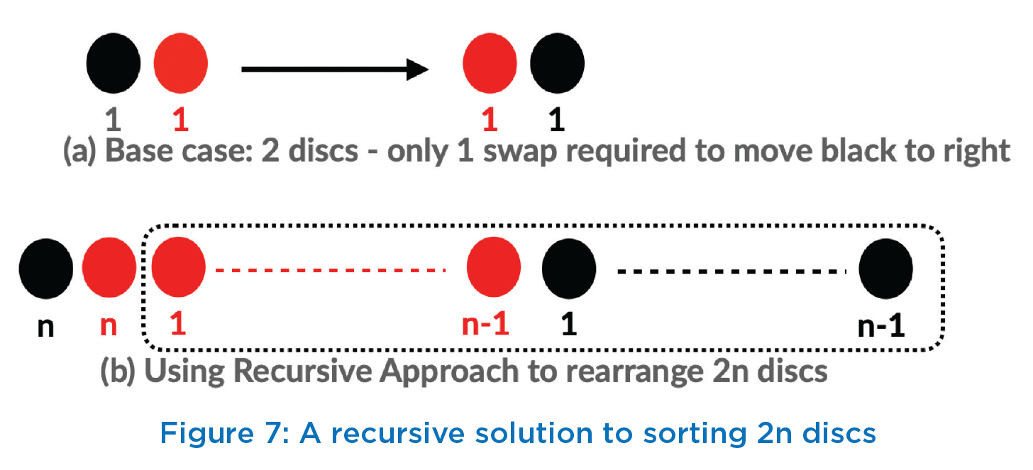
Is there an algorithm that achieves this minimum number of swaps? Again, recursion provides an elegant solution, as shown in Figure 7. Suppose this recursive algorithm makes ![]() swaps for
swaps for ![]() discs. As argued above,
discs. As argued above, ![]() 1, we first use recursion to sort the last
1, we first use recursion to sort the last ![]() discs using
discs using ![]() swaps, as shown in Figure 7(b). Next, we need n additional swaps to move the first (black) disc to the right of the n red discs. Hence, we obtain the recurrence
swaps, as shown in Figure 7(b). Next, we need n additional swaps to move the first (black) disc to the right of the n red discs. Hence, we obtain the recurrence ![]() =
= ![]() with the base case
with the base case ![]() Here again, a simple inductive argument can prove the equality
Here again, a simple inductive argument can prove the equality ![]()
![]() or the inequality
or the inequality ![]() Here again,
Here again, ![]()
There are two further pedagogically interesting points we would like to make about this puzzle. First, this problem can also be solved iteratively using Bubble Sort, which is familiar to most computer science students. Bubble Sort swaps adjacent values that are out of order, and this will require ![]() swaps as well. However, students once again have the opportunity to recognize the succinctness and beauty of the recursive solution.
swaps as well. However, students once again have the opportunity to recognize the succinctness and beauty of the recursive solution.
Second, there are many other ways of recursively solving the problem. For instance, it is immediately clear by symmetry that the algorithm could recursively sort the first ![]() discs and then handle the remaining
discs and then handle the remaining![]() discs by swapping the last red disc leftwards. More generally, the algorithm could solve two recursive sub-problems. For any
discs by swapping the last red disc leftwards. More generally, the algorithm could solve two recursive sub-problems. For any ![]() recursively sort the first
recursively sort the first ![]() discs to obtain a block of m red discs followed by a block of m black discs, then recursively sort the remaining
discs to obtain a block of m red discs followed by a block of m black discs, then recursively sort the remaining ![]() discs to obtain a block of
discs to obtain a block of ![]() red discs followed by a block of
red discs followed by a block of ![]() black discs, and then swap the first block of m black discs with the second block of n – m red discs. The two recursive solutions above are special cases of this more general algorithm, with
black discs, and then swap the first block of m black discs with the second block of n – m red discs. The two recursive solutions above are special cases of this more general algorithm, with ![]() respectively. In this general case, we obtain a more complex recurrence relation:
respectively. In this general case, we obtain a more complex recurrence relation: ![]() but the base case remains
but the base case remains ![]() You can show (by induction, of course) that for all choices of m,
You can show (by induction, of course) that for all choices of m, ![]()
Game 1: Nim
Next, we introduce students to non-linear recursion using the simplest version of the ancient game Nim ![]() In this game, there is a single pile of N discs and two players take turns to remove discs from the pile. On their turn, each player must remove either
In this game, there is a single pile of N discs and two players take turns to remove discs from the pile. On their turn, each player must remove either ![]() discs, and the player who picks up the last disc wins. (There are many other interesting variants of Nim!) A simple instance of this game with a pile of
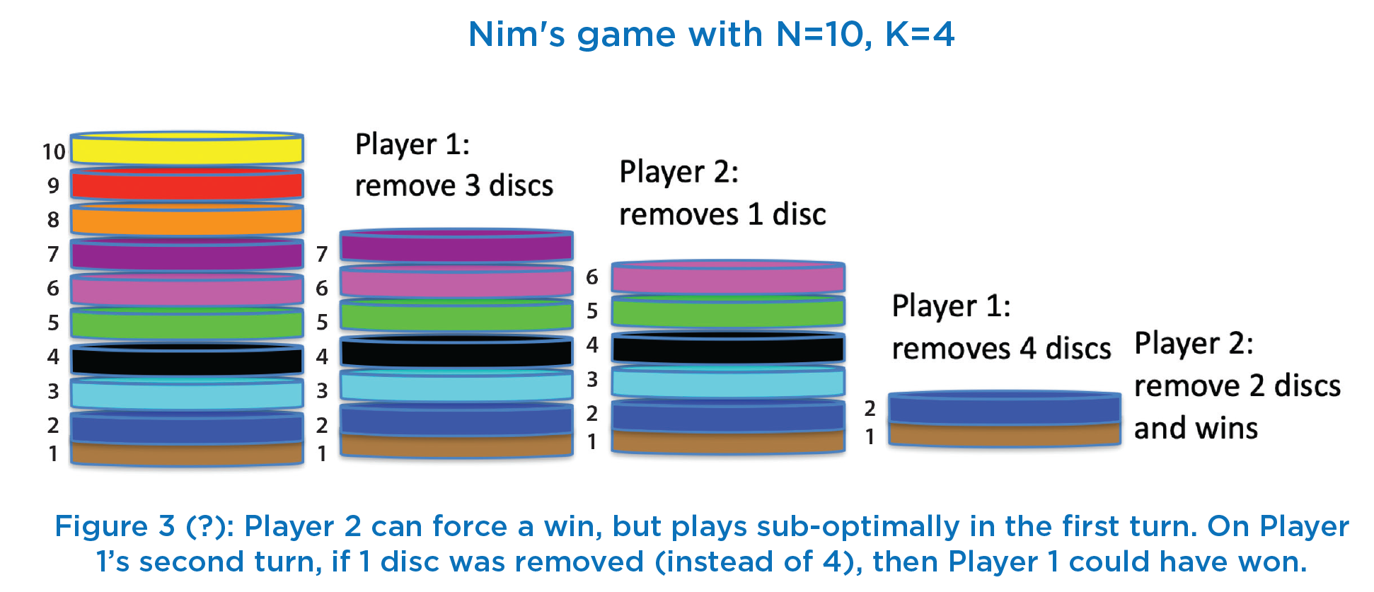
discs, and the player who picks up the last disc wins. (There are many other interesting variants of Nim!) A simple instance of this game with a pile of![]() is shown in Figure
is shown in Figure ![]() Here Player 1 first removes 3 discs and Player 2 removes 1 disc (this is a poor choice, as we shall see later). Next, Player 1 removes 4 discs (again a poor choice) and Player 2 wins the game by removing the 2 remaining discs. At this point, you are requested to play this game yourself with anyone else and see if you can work out a winning strategy for any
Here Player 1 first removes 3 discs and Player 2 removes 1 disc (this is a poor choice, as we shall see later). Next, Player 1 removes 4 discs (again a poor choice) and Player 2 wins the game by removing the 2 remaining discs. At this point, you are requested to play this game yourself with anyone else and see if you can work out a winning strategy for any ![]()
In class, we begin by restricting ![]() Thus, each player has only two options: remove 1 disc or remove 2 discs. We encourage students to work out an algorithm for determining which player wins (assuming both play optimally), given the initial number of discs N. Most students quickly work out that there are two base cases:
Thus, each player has only two options: remove 1 disc or remove 2 discs. We encourage students to work out an algorithm for determining which player wins (assuming both play optimally), given the initial number of discs N. Most students quickly work out that there are two base cases:
Player 1 wins if ![]() since Player 1 can remove all N discs. At this point, students may be tempted to examine larger values of N one at a time. If they do, they will quickly observe a pattern: Player 2 wins whenever N is a multiple of 3, and Player 1 wins otherwise. This leads to a trivial non-recursive algorithm, so we pause the conversation and discuss the general case when
since Player 1 can remove all N discs. At this point, students may be tempted to examine larger values of N one at a time. If they do, they will quickly observe a pattern: Player 2 wins whenever N is a multiple of 3, and Player 1 wins otherwise. This leads to a trivial non-recursive algorithm, so we pause the conversation and discuss the general case when ![]()
We point out that the current player has two options:
either remove 1 disc (in which case the opponent is left with ![]() – 1 discs), or remove 2 discs (in which case the opponent is left with
– 1 discs), or remove 2 discs (in which case the opponent is left with ![]() – 2 discs). Clearly, each player should choose an option that results in their own victory. We provide students with a few small hints. First, if the current player is Player p (where p is either 1 or 2), then the opponent is Player (3 –
– 2 discs). Clearly, each player should choose an option that results in their own victory. We provide students with a few small hints. First, if the current player is Player p (where p is either 1 or 2), then the opponent is Player (3 – ![]() ). Second, their recursive algorithm should take two arguments N and p, and should return the winner (either
). Second, their recursive algorithm should take two arguments N and p, and should return the winner (either ![]() or 3 –
or 3 – ![]() ). A correct recursive algorithm for determining the winner is shown in Table 3. Notice that there are two recursive calls on Line 4, which is non-linear recursion.
). A correct recursive algorithm for determining the winner is shown in Table 3. Notice that there are two recursive calls on Line 4, which is non-linear recursion.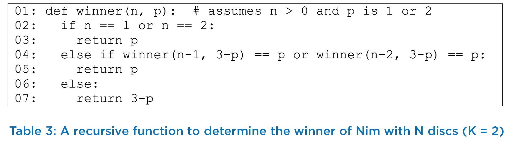
Finally, we wait until students point out that there is a much simpler and far more efficient algorithm in terms of both time and space based on the observed pattern noted earlier (a similar pattern can be observed for other values of K). Thus, we conclude by noting that an elegant recursive algorithm may not always be the most efficient algorithm for a given problem.
Apart from the challenge of tracing recursive code, two other key challenges for students are to formulate recursive algorithms to solve problems, and to accurately implement these algorithms. We will defer our discussion of this challenges to the next article.
We should do more non-linear recursion, such as:
Next article we will take some example using more complex examples and discuss the use of Master Theorem to derive the recurrence equation. We will further, discussion Binary searching using a novel game explaining binary search.