
Introduction
In our day-to-day life, we often use short form of words or codes (or mnemonics) to represent the words or phrases. We all use internet and any website domain in general today has two letter suffix code to represent the country where the company (owning the website) is present. For example, .in is for India, .jp for Japan, .uk for United Kingdom etc. The United States of America is an exception where most of the companies don’t use the suffix .us. All such US based entities have domain suffix as .com for company (or business entities), .edu for Educational Institutes, .org for organizations, .gov for US government etc. In general, when assigning codes (mnemonics/abbreviations etc) to words we use, it is our tendency to use shorter codes for more frequently used words and longer codes to less frequently used words. Similarly, when we make long distance landline phone call in India, shorter two digits STD codes are assigned to larger cities, where most people reside and have large number of phone connections, and longer codes are assigned for smaller cities. For example, STD (Subscriber Trunk Dialing) codes for Delhi, Mumbai, Chennai, Bangalore respectively are 11, 22, 44 and 80, whereas Jaipur (Rajasthan), Mysore (Karnataka), Madurai (Tamil Nadu) have their corresponding STD codes as 141, 821, 452. Further, the lesser populated smaller cities have longer codes even up to 6 or 7 digits.
We all use computers in daily life, and keyboard provides a basic and essential interface to work with computers. These input characters are stored with ASCII encoding using 8 bits (it was initially 7 bit) [1] . For example, character ‘A’ is encoded as 0x41 and ‘a’ is encoded as 0x61. All the ASCII characters are encoded with fixed length of 8 bits. This encoding is called Fixed Length Encoding.
In our daily use of English language, all of 26 alphabets do not appear equal number of times in any written text or spoken sentences. The letters ‘A’, ‘E’ and ‘I’ appear lot more often and letters ‘Z’ and ‘Q’ appear a smaller number of times. Thus, for efficiency reasons, we would like to assign shorter codes for frequently occurring characters and longer codes for those characters which occur infrequently. This was the core idea in designing Telegraph codes invented by Samuel Morse in 19th century. In this Morse Codes [2], each letter (26 alphabets and 10 digits) is represented by sequences of dot(.) and dash (-). The most frequently occurring character ‘E’ is denoted by single dot (.) and letter ‘A’ is represented by a dot followed by a dash (.-); letter ‘I’ is assigned two dots (..). The less frequently occurring letters such as ‘Q’ is assigned ‘--.-‘ and letter ‘Z’ is assigned ‘--..’. Since different size of encoding units are used for different characters, this is referred to as variable length encoding.
When we use variable length encoding, it poses the problem of distinguishing one character from other. For example, in Morse codes, encoding of ‘I’ starts with one dot (.) which corresponds to full encoding of letter ‘E’ and thus it requires some mechanism to ensure that letter ‘I’ is not decoded as ‘EE’. For this reason, Morse code uses a separator (equal to 3 units spaces) between two characters, which becomes an overhead thereby adding to communication cost. The other approach would be to design the variable length encoding in such a way that we avoid use of separators. This would require that encoding of any letter does not become prefix of code of another letter. A practical example of such encoding is used by Indian Telecom department to assign STD (Subscriber Trunk Dialing) codes and by International Telecommunication Union (ITU) to assign ISD (International Subscriber Dialing) codes. The country code of USA is single digit 1 whereas country code of India is 91. All these codes are such that code of any country (or city within country) does not appear as prefix of ISD code of other country (or city in that country). If codes would overlap, it would not be possible to route the calls to correct destination. Such encoding scheme is called Prefix-free encoding. This approach of prefix free variable length encoding provides shorter code length on the average compared to fixed length encoding and is one of the popular and efficient technique used in data compression.
The challenge in variable length encoding lies in generating such codes while complying with the following two requirements: a) shorter code for more frequently used cases, and longer codes for less frequently used cases i.e. length of code in some way is inversely related to frequency of occurrence, b) no code should appear as a prefix of another code. Huffman codes provides such a mechanism, and is named after David Huffman, who invented this scheme in 1952. [3]
Puzzle for Huffman Coding
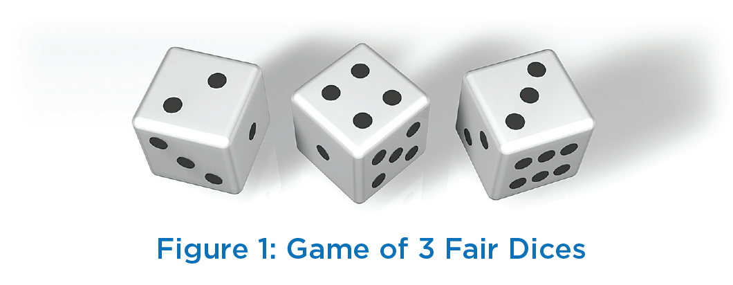
Adhering to the theme of GALA approach in this series of articles [4], we would like to start with the following puzzle/question. Consider a Gaming Arcade where one of the game counters offers a game of 3 dices and correctly guesses the sum of top faces. The operator asks you to throw three fair dices (shown in Figure 1) with each having their faces marked from 1 to 6 dots. The operator offers to guess the sum of dots on top face on 3 dices. For example, the sum value of top face of 3 dices as shown in Figure 1 corresponds to 9 (=2+4+3). The game operator charges a fees of Rs 19 to participate in the game but entices you to earn more money than the game fee.
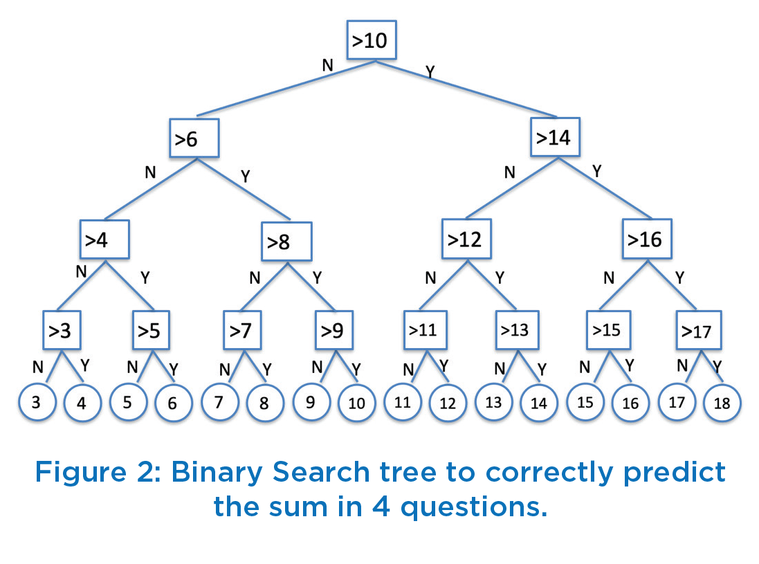
The game is played as follows. You throw 3 dices in private (which operator does not see) and note the sum. The game operator will ask you a series of yes/no type of questions i.e. question can only be answered either Yes or No. The operator pays you back Rs 5 for each Yes/No question being asked. Game will end only when operator has correctly predicted the sum value. Thus, if operator ends up asking 4 questions, the player will get back Rs 20 and make a profit of Rs 1 and loss to operator is Rs 1. As can be easily seen that minimum sum value is 3 (=1+1+1) and maximum sum value is 18 (-6+6+6) i.e. sum values ranges from 3 to 18, making it a total of 16 values. Any course on Data Structure always includes a Binary Search algorithm, which says that given any N numbers arranged in sorted order, a search can always be completed in log2N time. Thus, if operator were to use binary search mechanism, this sum can always be correctly predicted in 4 attempts (log216=4 as 24=16). For example, for the sum value 9 (as in figure 1), the operator would ask the following four questions to predict the sum correctly.
After the 4th question, the operator correctly tells you that sum is 9 (as the sum can either be 9 or 10 before 4th question is asked). Thus, by asking 4 questions operator correctly predicts the sum value. However, operator has incurred a loss of Rs 1 since game fee was Rs 19 and ended up paying Rs 20. So, using the strategy of binary search, the operator will always lose money. A typical logical sequence of questions is shown as a decision tree structure in Figure 2 which corresponds to Binary Search technique. If the game fee is set to more than Rs 20, than no participant will play the game since participant can easily work out the logic of binary search. Keeping the game fee at Rs 20 is meaningless since operator does not gain any profit and simply wastes effort. So, the game fee has to be kept less than Rs 20 to make it enticing for the player to participate. Thus, we have defined the game fee to be Rs 19/-. Essentially, the game fee should be set to a value which is less than 4 times the pay back money per question. So, it should not be obvious to participant how the operator will make money.
To develop a better understanding of the problem, you are requested to pause the reading of this article and workout the strategy for the operator so that it can make money per game instance on the average while keeping it attractive to participants. This implies that for some game instances, operator will incur loss and for other game instances it will make profit. However, when a number game instances have been played, it should make a profit overall. Any strategy to be developed cannot change the rules of the game i.e. operator can ask only those questions which can be answered in either Yes or No. For example, a question can be “Is the sum value equal to any of 1,3,5,7,9,11,13,15 or 17”? Since this question can be answered in Yes/No, and hence is a valid question. We need to devise only those strategies which would result in asking less than 4 questions on the average per game to correctly predict the sum.
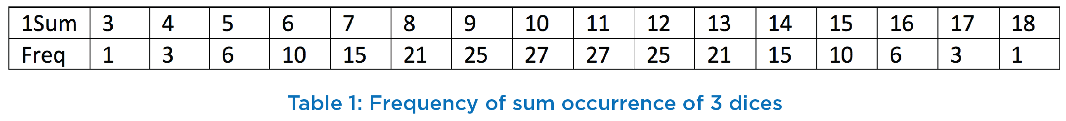
Let us look at a possible approach. The total possible outcome space of 3 dices is represented by triplet (a,b,c) where each of a, b and c can take value between 1 to 6. Thus, a total possible outcome space would have 216 (=6*6*6) combinations represented by {(1,1,1), (1,1,2),…, (1,1,6), (1,2,1), …, (1,2,6), …, (6.6.6)}. Considering that dices are fair, and thus each outcome is equally likely, the frequency of each sum value out of 216 possible combinations is given in Table 1. The sum value 1 would correspond to (1,1,1) and sum value 18 would correspond to (6,6,6). The sum value 10 and 11 occurs 27 times. Few instances of outcome space of sum value 27 are {(1,3,6), {1,4,5), (1,5,4), (1,6,3), (2,2,6), …, (6,2,2), (6,1,3)}.
Given this frequency distribution of sum values, the challenge lies in designing our questions so that number of questions asked is less than 4 on the average in a game instance. If 4 or more questions are asked in a game, operator would lose money in that game. Intuitively, one would like to start with questions that involve sum being 10 or 11 since these sum values have highest frequency. These two questions asked in any order have only 25% (-54/216) success and would forego Rs 10, more than 50% of the game fee.
Before we build our solution, let us revisit the binary search model and analyze the reasons why it failed to work. In binary search mode, correct prediction of each sum requires exactly 4 questions to be asked, as can be seen by traversing the path from root of the binary decision tree in Figure 2. For example, to correctly predict the sum being 16, the sequence of 4 questions that will be asked correspond to >10 (Yes), >14 (Yes), >16 (No), and >15 (Yes). This corresponds to 4 bits encoding where 1 represents Yes answer and 0 represents No answer. Each bit position corresponds to one question being asked. Thus, encoding for sum value 16 would correspond to binary number 1101 (Yes, Yes, No, Yes). The binary number 1101 is equal to 13 which corresponds to 13th sum value of 16 in the range 3..18. Thus, binary number 0000 would correspond to
sum value 3, and binary number 1111 would correspond to sum value 18. The binary search approach gives equal weightage to all sum values irrespective of their frequency of occurrence. It uses fixed length encoding and that is the reason this approach does not work for the Game vendor.
The feasible solution needs to use variable length encoding and it must be prefix free. Since each question being asked needs to be answered either Yes/No, the solution has to follow the binary tree path where Yes would imply follow one path and No would lead to another path. The variable encoding would assign shorter codes to sum values with highest frequency, such as 10 and 11. This encoding would assign longer codes to less frequently occurring sum values such as 3 and 18. The mechanism of Huffman Tree construction provides such a solution and we will develop a Huffman tree for this problem [3].
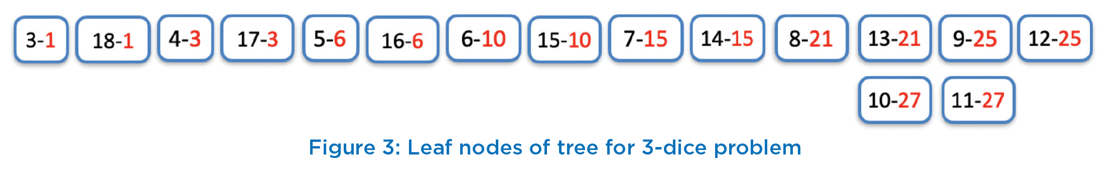
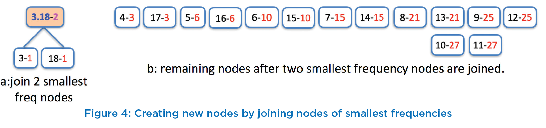
The solution works as follows. Write all the sum values (of 3 dices) in ascending order of their frequencies as shown in Figure 3. Each sum value is represented by a node (actually a tree with just 1 node) with its label consisting of sum value and frequency count. Thus, Figure 3 represents a forest with 16 trees. The label is represented as “a-b”, where “a” corresponds to sum value and “b” corresponds to frequency of sum value “a” as per Table 1. In the Figure 3, nodes are arranged in ascending order of their frequencies.
First step in our solution is to take two nodes with smallest frequency values and join them to create a new node with a cumulative frequency value i.e. equal to sum of the frequencies of underlying two nodes. Similarly, label of the new node is created by concatenating the sum values of underlying nodes and adding the cumulative frequency. In our case, first two nodes being considered are (3-1), and (18-1) and therefore, the new node will be represented as (3.18-2) with “3-18” as the sum values and 2 as its frequency. This is shown in Figure 4a, and remaining nodes are shown in Figure 4b. Each newly created node becomes root of the tree with two nodes as its left and right children. Among the two nodes, the node with lower frequency will become the left child and other node with higher frequency value would become the right child.
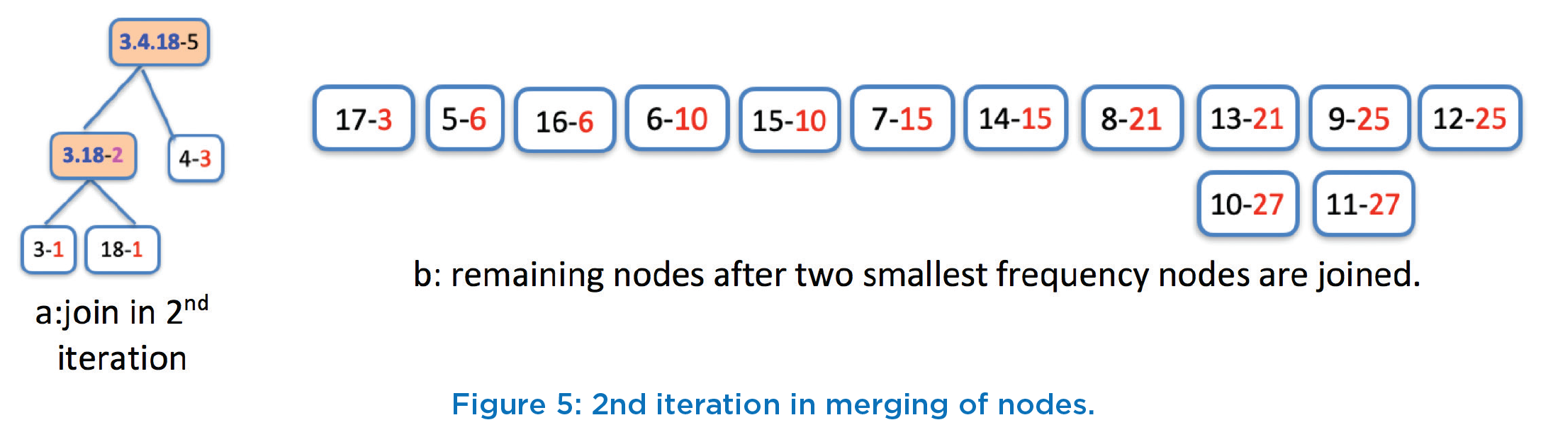
Repeat the above process of joining two nodes with smallest frequency values to create a new node with cumulative frequency value till all nodes are joined to become a single tree. Thus, in 2nd iteration, the next two nodes as per Figure 4 are “3.18-2” and “4-3” or “3-18-2” and “17-3”. Since there are two choices, either one of these can be taken since both choices will give same cumulative frequency value of 5. Let us take the first choice and proceed with nodes “3.18-2” and “4-3”. After joining these two nodes, the resulting node would be “3.4.18-5” (for ease of convenience we are keeping the sum values in the label in ascending order after concatenation). The result after this iteration is shown in Figure 5a and remaining nodes that are yet to be processed are shown in Figure 5b.
In our 3rd iteration, the next two nodes to consider are “17- 3” and “3.4.18-5” corresponding to smallest frequencies 3 and 5. This new created node after joining these two nodes would have the sum values as “3.4.17.18” and frequency value as 8 (=3+5). Thus, we will depict this node as “3.4.17.18-8”, as shown in Figure 6a. It can be easily seen that sum value part of the label of root node of tree corresponds to concatenated sum values of all of its leaf nodes. In the 4th iteration, next two nodes with smallest frequency values among all nodes (including new created nodes and existing nodes) are “5-6” and 16-6” with their frequency value as 6. Thus, next node will be created with label as “5.16-12” as shown in Figure 6b. Remaining nodes are shown in Figure 6c.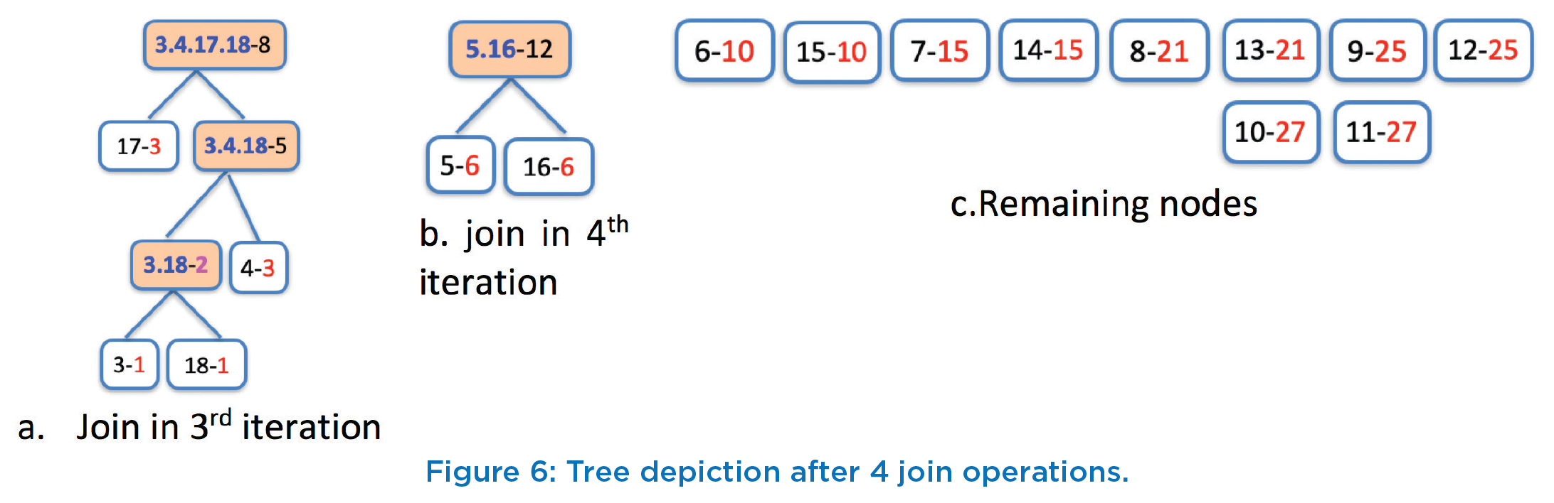
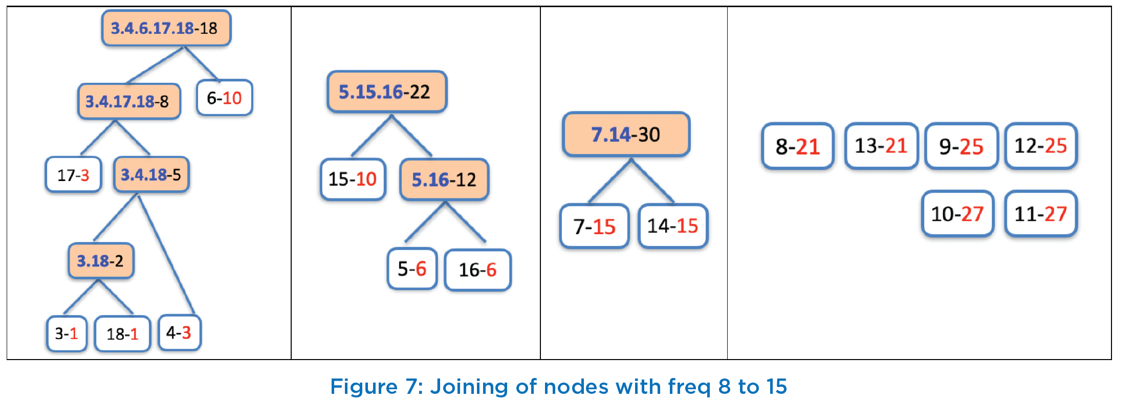
Continuing in this way, in the 5th iteration, next two nodes corresponding to smallest frequency will be “3.4.17.18-8” and “6-10” (instead, we can alternately consider node “15- 10” as well) and new created node after joining these two would be labeled as “3.4.6.17.18-18”. In 6th iteration, nodes with least frequency will be “15-10” and “5.16-12” and new created node after joining these two would have the label as "5.15.16-22” with frequency value of 22. Similarly, in 7th iteration, next two nodes with least frequency values are “7-15” and “14-15” and joining of these two nodes result in creation of node “7.14-30”. The status of all nodes after these 5th, 6th and 7th iteration is shown in first 3 columns of Figure 7. The last column shows remaining nodes that needs to be processed next.
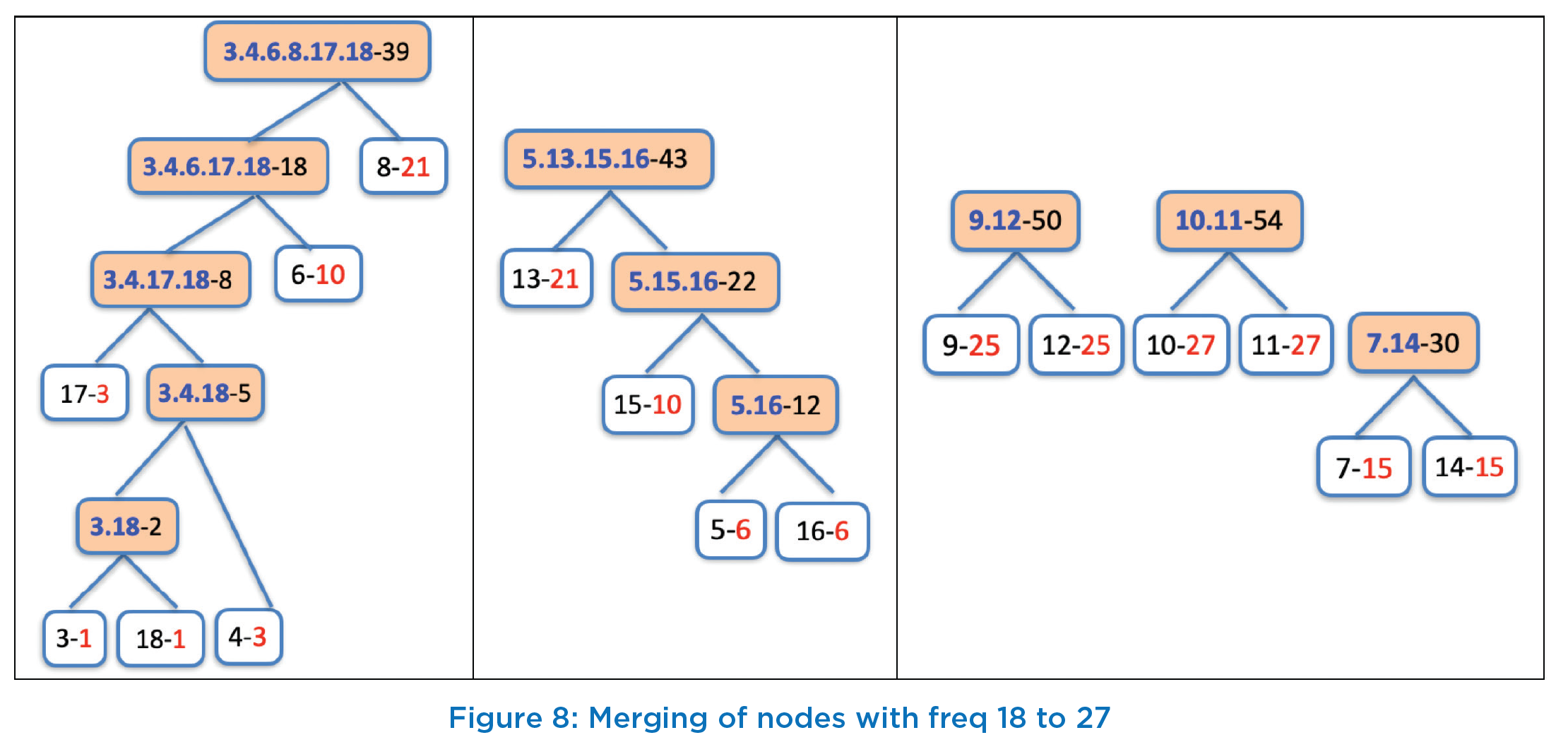
After 7th iteration, as per Figure 7, two lowest frequencies are 18 with label “3.4.6.17.18” and 21 with two nodes “8-21” and “13-21”. For simplicity, we will take node “8-21”. Thus, in 8th iteration, we create a node with label “3.4.6.8.17.18- 39” with frequency value of 39 (=18+21). This is shown in first column of Figure 8. In 9th iteration, next two nodes to consider for joining are with frequency 21 (“13-21”) and 22 (“5.15.16-22”) and create a new node with label as “5.13.15.16-43” as shown in 2nd column of Figure 8. Similarly, the nodes “9-25” and “!2-25” are joined in 10th iteration to create a node with label “9.12-50”, and then node “10-27” is joined with node “11-27” in 11th iteration to create a node with label “10.11-54” and is shown in 3rd column of Figure 8.
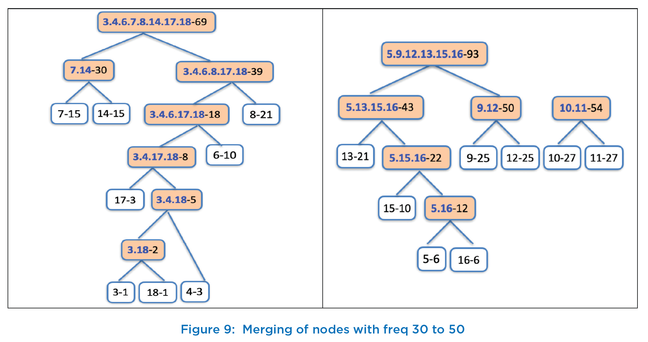
At this stage, though we do not have any more original nodes with single sum value, but we will continue the process of picking two nodes with least frequencies and join them. Thus, in next iteration, the next node will be created with the label “3.4.6.7.8.14.17.18-69” with cumulative frequency of 69. This is shown in first column of Figure 9. 2nd column of Figure 9 shows the next new node with label “5.9.12.13.15.16-93” which is created by joining nodes “5.13.15.16-43” and “9.12-50” in 13th iteration.
We now have just 3 trees with frequencies as 54, 69, and 93. We still need to work on two more join operations to create a single tree. Thus, next we join nodes “10.11-54” and “3.4.6.7.8.14.17.18-69” to create a new node with frequency of 123 and label as “3.4.6.7.8.10.11.14.17.18-123”. This is shown in first column of Figure 10 and previously created node in right column of Figure 10. The last operation is to join these two nodes, and thus in our last and 15th iteration, we create a new node with frequency as 216 (=123+93) with label that contains all the sum values i.e., label of root of Huffman tree is “3.4.5.6.7.8.9.10.11.12.13.14.15.16.17.18-216” and 216 is the total number of possible combinations that can be achieved by throwing 3 dices computing the sum of top faces. This Huffman tree is shown in Figure 11
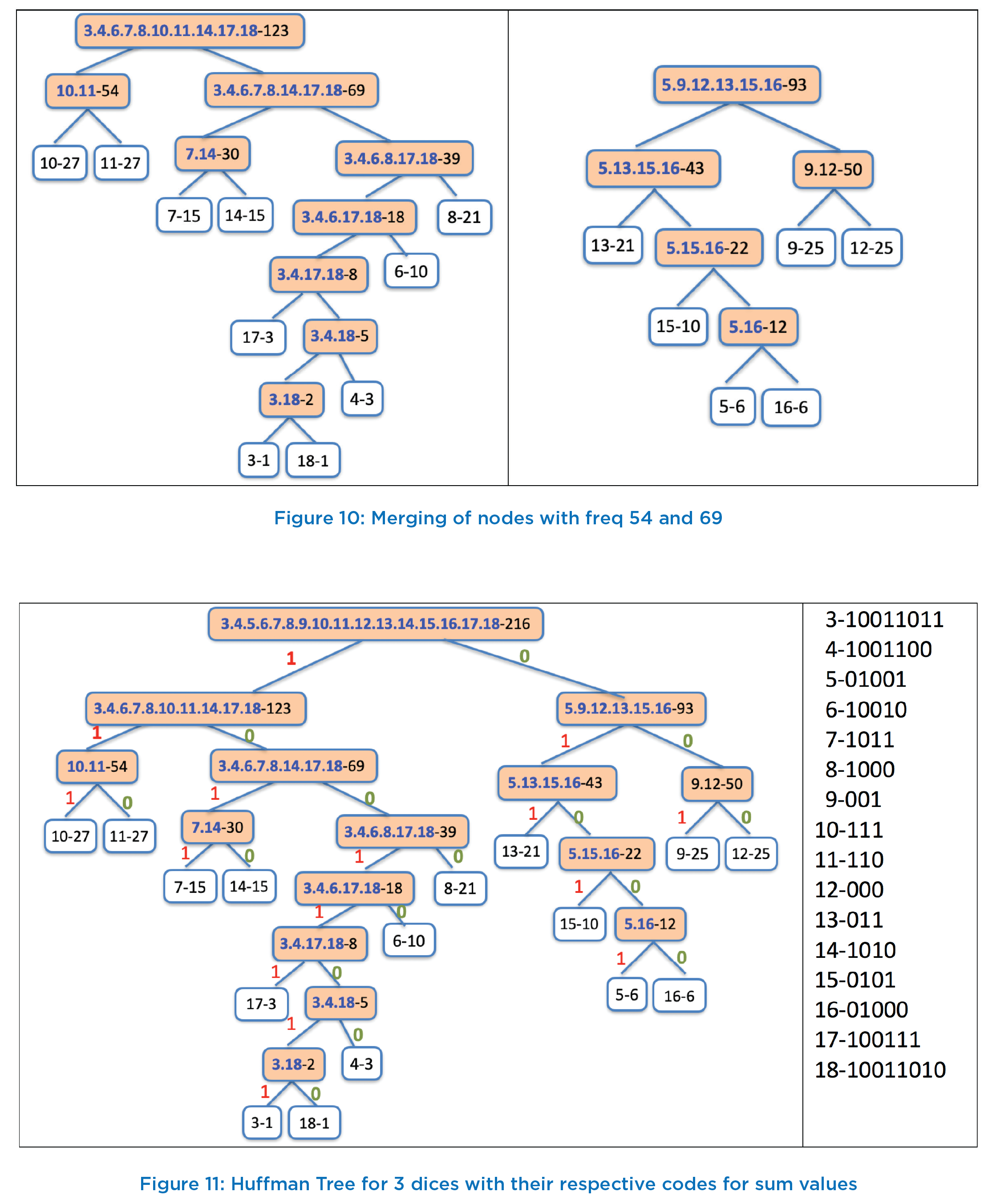 After the Huffman Tree is built for 3-Dices game, next task is to assign prefix free variable length codes to each of sum. To arrive at the codes for each sum value, we start at the root node (with label “3.4.5.6.7.8.9.10.11.12.13.14.15.16.17.18.- 216” and traverse the tree, and mark each right edge with “0” and mark each left edge with “1”. Thus, the right edge connecting the node “5.9.12.13.15.16-95” with root node is marked as “0” and left edge connecting the root to the node “3.4.6.7.8.10.11.14.17.18-123” is marked as 1. Proceeding in this way, we mark all the edges. This marking process stops when we reach leaf node in the traversal. The leaf node will correspond to actual value with its frequency of occurrence. The marking of each edge of Huffman Tree is shown in Figure 11.
We assign the variable length codes to each sum value as follows. Traverse the path from root node to this leaf and catenate all edge marks along the way. Thus, the node “10- 27” is assigned the code as 111, as it follows all the left edge starting from root node i.e. traversal path from root to this leaf node follows Left(1)-Left(1)-Left(1). Similarly, the node “11-27” is assigned the code 110 as the traversal path to this node is Left(1)-Left(1)-Right(0). These are the nodes with shortest length code in this tree with code length equal to 3. Consider the path from root to the two initial nodes “3-1” and “18-1” with which we started the join process. The traversal path from root to the node “3-1” is Left(1)- Right(0)-Right(0)-Left(1)-Left(1)-Right(0)-Left(1)-Left(1), and thus the code 10011011 is assigned to sum value 3 i.e., node “3-1”. Similarly, sum value 18 (node “18-1”) is assigned the code 10011010. Both these sum values have a frequency count of 1 (out of 216) and gets assigned the longest code of length 8. The codes for all sum values can be assigned in in similar fashion by following the path from root to the corresponding leaf node for that sum value. These codes for all sum values are shown in 2nd column of Figure 11.
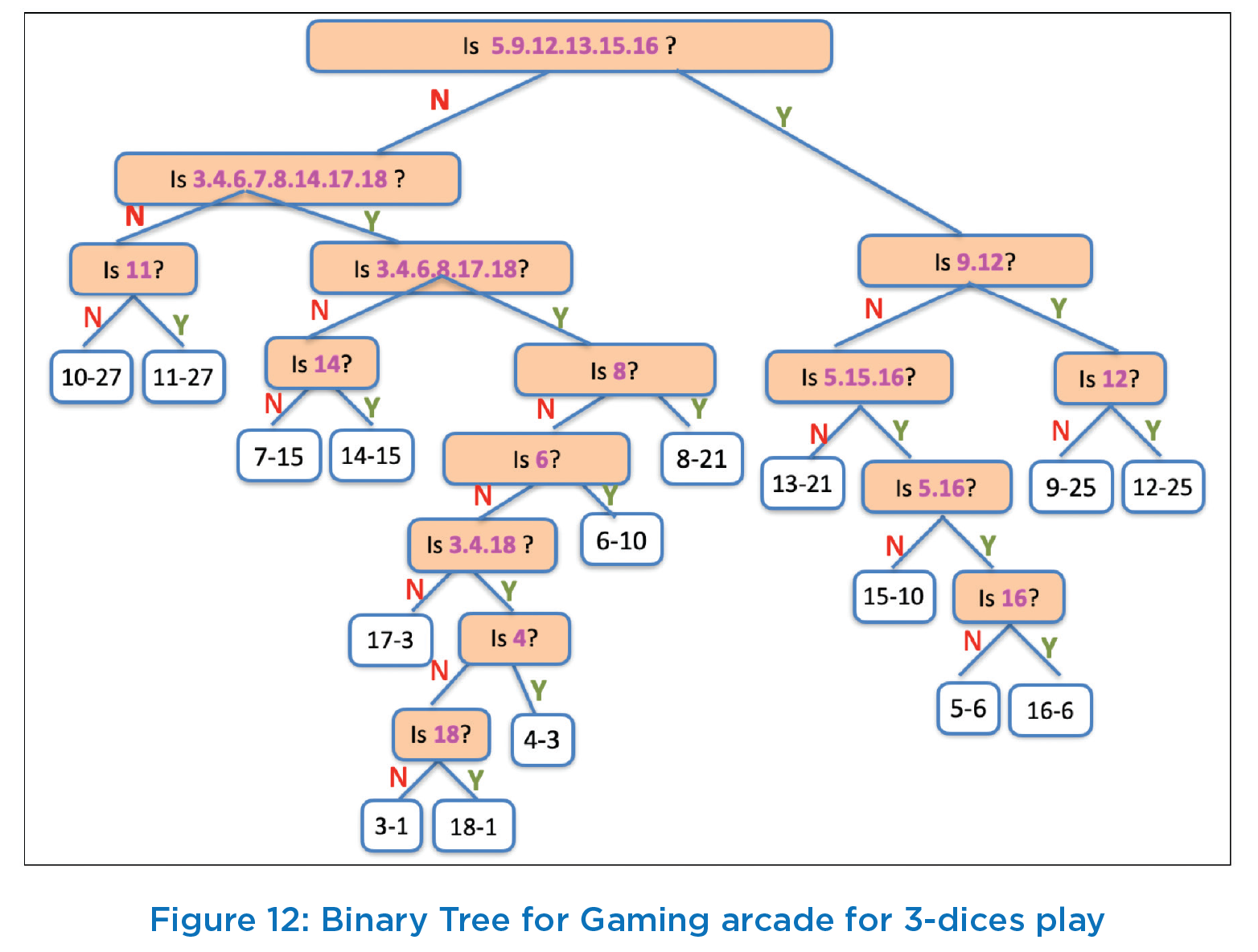
Our next task is to address the question that we started with i.e., how does Gaming arcade makes money considering that questions have to be such that these can only be answered Yes or No. So, we work out a mechanism that will identify the questions to be asked. In the Huffman tree of Figure 11, we start at the root, ask the first question, follow the right edge on Yes answer and follow the left edge on No answer. Keep repeating this process till we reach the leaf node which Is identified by series of these questions. At intermediate nodes, question is formed as follows. At each intermediate node, took at the node label reachable by right edge and ask the question “Is the sum value of 3 dices among any of v1,v2,…vk”? (where v1,v2,… vk correspond to sum values in label of right child i.e. node reachable by right edge). Thus, starting at the root as shown in Figure 12, i.e., the first question asked will be “Is the sum of 3 dices among any of 5,9,12,13,15,16?”. If the answer is Yes, follow the right edge to reach the next intermediate node “9.12-50”, and ask the second question “Is the sum of 3 dices among any of 9,12”?. If the answer is Yes, again, we traverse the right edge, look at node label and ask the 3rd question: “Is the sum 12?” If the answer is Yes, we have correctly predicted the sum to be 12. If the answer to 3rd question is No, then we would follow the left edge and correctly predict the sum as 9. For both these sum values of 9 and 12, only 3 questions are asked and thus Gaming arcade pays back only Rs 15 against Rs 19 as game fees and thus makes a profit of Rs 4.
Analysis
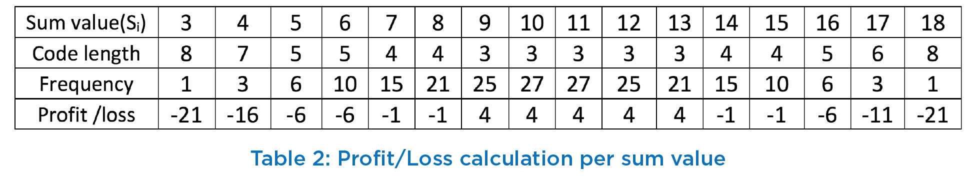
We will now analyze why this Huffman Tree based approach works i.e. makes profit for Gaming Arcade. Consider the binary code for any sum value. The value ‘0’ corresponds to question being answered in Yes, and value ‘1’ corresponds to No answer. The number of questions needed to be asked for a given sum is equal to number of digits in the code corresponding to the sum. This means that all those sum values whose code length is 3, gaming arcade would make a profit of Rs 4 (=19-5*3). For all other codes, gaming arcade would lose money depending upon the code length. For the sum value with code length of 4 (e.g., 7,8,14,15), Arcade would incur a loss of Rs 1 (=5*4-19). Gaming arcade incurs maximum loss for sum values of 3 and 18 having code length of 8. For these two sum values of 3 and 18, Gaming arcade would lose Rs 21 (=8*5-19). Table 2 summarizes the profit made or loss incurred associated with sum value in one game instance. However, since the 3 dices are fair, the probability of occurrence of a sum value is equal to its frequency of occurrence divided by 216 (the size of total outcome space). Thus, average profit/loss per game to the gaming arcade would be equal to Rs 1/216*(- 21*1-16*3-6*6-6*10-1*15-1*21+4*25+4*27+4*25+4*21- 1*15-1*10-6*6-11*3-21*1) = Rs 184/216 = Rs 0.85. Thus, on the average, gaming arcade makes a profit of Rs 0.85. This approach works because profit made in sum values 9,10,11,12,13 with highest frequencies of occurrences overcomes the loss incurred for other sum values.
Huffman Algorithm and Compression Ratio
A simple examination of Huffman codes for 3-dices problems shows that all codes are prefix-free i.e., no code is a proper prefix of another code. This can be easily understood from the traversal path since code termination occurs at a leaf node, and for any code to be prefix of another code, path cannot terminate at that node. Let us now analyze the compression ratio achieved by Huffman coding for our example. Compression ratio provides efficiency variable length encoding over the fixed length encoding. In our example, for fixed length binary coding, the length of each code is 4. When using prefix free variable length encoding, the average code length will be computed by multiplying the code length with its probability occurrence and computing sum of all such terms. Let Ci represent the code for ![]() sum value Si, then prob(Si) is equal to its frequency divided by 216. For example, for
sum value Si, then prob(Si) is equal to its frequency divided by 216. For example, for ![]() is 8, and probability
is 8, and probability ![]() Thus, average code length would be given by
Thus, average code length would be given by ![]()

When constructing the Huffman Tree, often we find more nodes with same frequency and we can choose either one. Each such choice would give a different Huffman Tree, and hence Huffman.
Algorithm does not guarantee unique tree. Thus, for a given set of values with their frequencies of occurrence, many Huffman Trees can be constructed. Researchers have conducted extensive experiments using Huffman codes using various data sets and found that compression ratio typically would range between 20% to 80% . The details of Huffman Algorithm can be found in [3] and any text book on Algorithms.
Summary
We have discussed a simple game or puzzle-based approach to explain practical use of Huffman coding. We have used an interesting number guessing game to explain the use of prefix free variable length encoding. One can few variations of this game to make it more enticing for the player. For example, notice that gaming vendor makes profit only for 5 sum values (i.e., 9,10,11,12 and 13) and incurs loss on 11 sum values. Thus, for 2/3rd of sum values, player earns profit and same can be advertised as an attractive proposition to participating players. Another variation can be to take the approach of reducing the losses. For example, when number of questions being asked becomes 5 or more, it can stop asking the questions. But to make the game enticing to participants, game vendor can advertise that if it cannot predict the sum correctly, it will pay back Rs 25. Thus, for sum values 3, 4, 17, and 18, it will pay back only Rs 25 instead of Rs 40, 35, 30 and 40 respectively, thereby reducing the losses. The average profit per game instance will then increase to Rs 1.12 from Rs 0.85. To avoid monotony of the same set of questions, game vendor can make all possible Huffman Tree. In each new game, the vendor uses different set of questions based on other Huffman Trees. That way it would become challenging for any player to understand the logic being used.
The Huffman algorithm provides efficient encoding for a given distribution, though it may not always be optimal. It provides optimal codes if all the frequency distributions follow the powers of two probability and all the values in the set are independent. In other cases, there are other algorithms that can provide better encoding. Huffman coding is widely used in file compression applications. There are other applications areas, for example, Gaming applications, Decision Tree problems etc. where Huffman coding can be used.
As an exercises, readers of this article are requested to take any paragraph text (e.g. any text from this article itself) of their choice, and compute the frequencies of each letter and build the Huffman tree and compute the compression ratio w.r.t. fixed size 7 bits encoding of ASCII character set.
R E F E R E N C E S
1. American Standard Code for Information Interchange (ASCII Table); https://www.asciitable.com/, last accessed January 2022.
2. Morse Codes. https://en.wikipedia.org/wiki/Morse_code, last accessed January 2022.
3. Anany Levitin, “Introduction to the Design and Analysis of Algorithms”, 2nd edition, Pearson Education.
4. Ram Rustagi, Viraj Kumar, A Gamified Approach to Learning Algorithms, ACS Journal on Advanced Computing and Communications, March 2021, Volume 5 issue 1. https://journal.accsindia.org/gala-a-gamifiedapproach- to-learning-algorithms/