1. Introduction

There is a frequently used phrase, which says that “80% of all information contains some geo-reference.” Hahmann and Burghardt [10] have reformulated this phrase using evidence to a “60% assertion.” Nonetheless, the geo-referenced data remains to be relatively more ubiquitous than non-geo-referenced data. Consider the NISAR (NASAISRO Synthetic Aperture Radar) mission [30], which the two space organizations are going to jointly launch in 2021. The mission is expected to generate around 85 TB of data daily [6]. The radar imaging satellite will be designed to use dual frequency for remote sensing for studying natural processes and estimating earth observations (e.g. biomass, surface deformation, soil moisture, etc.). The mission is estimated to gather about 140 PB in its 3-year mission.
Overall, the message is loud and clear that geospatial big data is going to stay and grow, more so. Hence, its analytics cannot be ignored. Li et al. [20] have discussed how visualization provides a class of methodologies to gain human insight to geospatial big data. Visualizations provide yet another channel for identifying outliers, building and verifying hypotheses, and most importantly, “seeing” dominant trends and patterns. Visualization as a domain has contributed towards techniques for summarization and exploration of data, as well as “computational steering”. Computational steering [29, 28] is the process of improving on computations by using intermediate data visualizations, which effectively influence the workflow. While computational steering is used in computational simulations, a more recent trend has been observed in the form of progressive visual analytics.

 

1.1 What is Visual Analytics and How is it Different from Visualizations?

Keim et al. [17] have defined visual analytics as a combination of conventional data mining and interactive  visualizations in a data analytic workflow, for understanding, inferences, and decision-making support for big data. In all interactive applications today, visualizations have paved the way for visual analytics. This evolution has happened because a stand-alone visualization or a group of visualizations carefully assembled together is no longer sufficient for making sense of the big data. Visual analytics processes, as shown in Figure 1, could be non-deterministic, as well, and form a feedback loop which terminates only when “visualization requirements” are met.

 

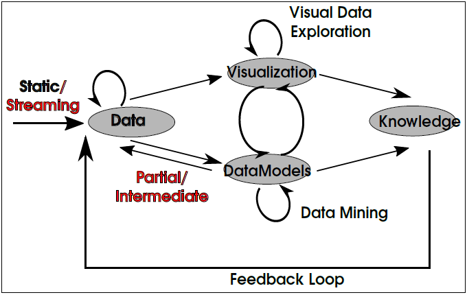
Fig. 1: The visual analytics workflow, as defined by [17], has been modified to include (a) streaming data; and (b) data feed from data mining. Use of streaming data leads to incremental visual analytics [31] and use of data in (b) leads to progressive visual analytics [33, 4].
A more recent concept, “progressive visual analytics,” [33], entails the use of visualization to study the “meaningful partial results” given out during the execution of data analytic workflow. Fekete and Primet [8] have proposed progressive analytics to be a synonym for “progressive computations for data analytics,” with consideration for low latency. Including visualizations to support progressive analytics, Badam et al. [4] have differentiated between progressive and incremental visual analytics – where the latter caters to data streaming [31]. Their prototype for “progressive visual analytics” combines both incremental as well as progressive visualization with algorithmic steering, i.e. iterative control over execution of a computational process [28].

1.2 Geovisualizations and Geovisual Analytics

For visual analysis, specifically, in geospatial applications, MacEachren and Kraak have introduced geovisualization [26] as an amalgamation of the areas of visualization, scientific computing, and geographic information systems (GIS) to make sense of geospatiotemporal data. MacEachren et al. [25] have defined the four functions of geovisualizations to be “explore, analyze, synthesize, and present.” They also have defined the space of  geovisualizations to be a cube with axes for task types, user types, and user interaction level.

In 2007, Andrienko et al. [1] have introduced the term geovisual analytics, setting the stage for its widespread usage as well as development. They have pushed forward the research agenda for “geovisual analytics for spatial decision support systems” and differentiated geovisual analytics from the regular visual analytics using three characteristics, namely, complex spatio-temporal nature of the data involved, multiple stakeholders, and tacit criteria and knowledge. They have illustrated the application of geovisual analytics in the example of emergency response in a disaster-affected region. Specifically, to plan the evacuation of people from the region, the planner needs information of the geography of the place, the road network, the hospital facilities en route, high-risk personnel, etc. We see that the problem blows out to be a multi-criteria optimization one. The decision making of the planner, in this case, may be alleviated by making inferences from different “slices” of the data. Visual analytics can also be used to study the dynamism in this example, say, we can progressively refine the solution using both the incoming streaming data of the evacuation process as well as partial results from other data mining process (Figure 1).

In this paper, we sample some of the popularly used geovisualizations in Sections 2 and 3, demonstrate geovisual analytics using a case study in Section 4, and finally articulate the research challenges in geovisual analytics. Geo-referencing makes the use of cartographic products an important element of the visualizations. Hence, we discuss map-based visualizations in Section 2, and other related visualizations in Section 3. The geovisualization techniques described in this paper are not exhaustive, however. For instance, we have not covered the role of information visualization techniques as well as user interactions in all of these visualizations. For details of these topics in the context of geovisualization, they can be found in parts in [2, 3, 12]. In the current article, we focus on discussing popularly used geovisualizations and move on to show how they influence geovisual analytics in a specific case study.

2. Map-Based Visualizations

Several of the standard geovisualizations use cartographic maps as contextual elements, owing to the geo-referential property of the data. We discuss most popularly used techniques using examples of visualizations of Singapore ¹, as shown in Figure 2:

Choropleth map: Choropleth map is a cartographic map where (political or other logical) partitions of regions are colored based on the color computed from the value of an attribute, e.g. population density, in that partition. A value of an attribute pertaining to a specific region is mapped to a color in a spectrum for a single attribute. The mapping of the value to a color involves a “transfer” function. Conventionally, this is a linear function, considering a trade-off between computations and accuracy. An example is a black-to-blue spectrum, mapped from minimum to maximum value of a function, the saturation of the blue component corresponds to the normalized value of the function.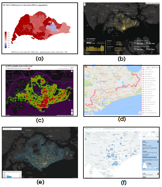

Fig. 2: Map-based visualizations of Singapore from http://www.viz.sg/:

(a) Districtwise heatmap of difference in vote share during the general elections in 2015;
(b)Location-wise heatmap of taxi availability during peak hour (8:45 pm) on December 15, 2017;
(c) Hotspot heatmap of taxi availability on October 4, 2017, at 11:40 am;
(d) Node-link diagram showing route of bus service-5 in Singapore;
(e) Isochrone map showing reachability by public transport for 15-minute increments from Raffles Place Singapore; and
(f) Symbol map using blue circles to uniquely represent projects of private home property being completed during 2016-17, where the size of the circle indicates number of units.

^[1] The visualizations of Singapore are available at the portal http://www.viz.sg

 

Hotspots: The density of a specific value is mapped to an entire region, based on the discrete values in the region. A kernel density estimation function is used to compute the density at all points, and they are colored depending on the density values. The hotspots are regions which show how the density decreases as one goes away from the hotspot. The hotspot uses a standard color spectrum, where it is usually rendered in red, which subsequently fades into orange, yellow, and green.
Network visualization: Networks are ubiquitously represented in the form of twoor three-dimensional geometric primitives (e.g., circles, spheres, triangles, etc.) for nodes, and one-dimensional geometric primitives (e.g., lines and curves) for the links between the nodes². Thus, networks are popularly represented using nodelink diagrams. The variations of the visualizations come from the differences in rendering of the nodes and links, and the graph layout of the network itself. In geospatial data, transport networks (road, rail, airlines, etc.) are represented using node-link diagrams. Map-based node-link diagrams constrain the location of the nodes to be rendered at its latitude-longitude location, as per the cartographic maps.
Isochrones: For transport networks, the visual representation of regions which can be arrived from a given point at the same time, show the reachability, and thus efficiency, of the network. One could thus mark the region reachable in, say dt amount of time, from a starting point. This can grow out to regions reachable in increments of dt time periods. Each of these regions are called an isochrone. Such visualizations can alternatively be constructed using distance as a measure, instead of time. Such visualizations are called iso-distance views.
Symbol map or glyph/icon-based visualization: Symbols, glyphs or icons are diagrammatic representations of associated attribute/property of the (discrete) point at which the glyph is placed. One of the most universally accepted glyph is an arrow for representing a vector or direction. Similarly, in the case of geospatial data, a specific attribute, say property taxes or population, can be represented as a circle, as a glyph, whose radius indicates the relative value. The transfer function used in choropleth map can be used for coloring the glyphs, thus encoding the values using color.
Three-dimensional visualization: Considering maps can be used as textures in computer graphics  applications, one could generate volumetric visualizations. A popular web-based earth observation visualization showing the global weather conditions and ocean surface currents is at http://earth.nullschool.net, samples of which are shown in Figure 3.
Even though a three-dimensional visualization requires extensive computations in comparison to its two-dimensional counterparts, it provides more intuition and dimensionality realism to geospatial data. Apart from the texture-based visualizations, this class also includes visualizations which show extrusions in the third dimension, from a plane with two-dimensional map texture, e.g. three-dimensional modeling of buildings on a flat/planar map of a city.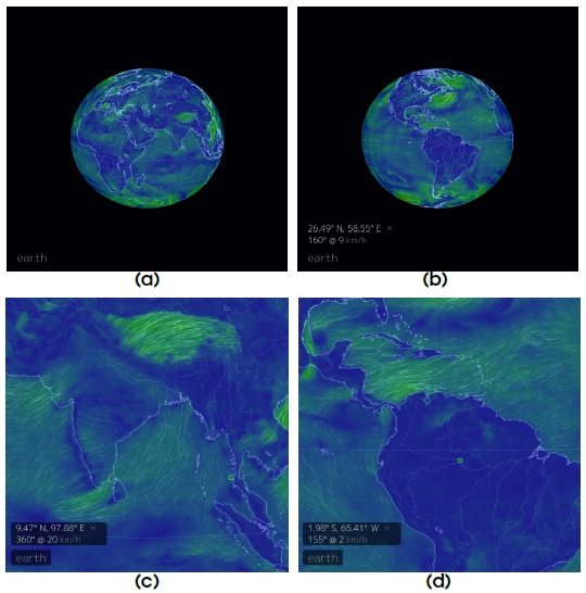

Fig. 3: Interactive three-dimensional visualization of global weather conditions and ocean surface currents at http://earth.nullschool.net which is updated every three hours using forecasts computed on supercomputers. Note the artistic rendering in the visualization of the map of the global wind directions and magnitude in

(a) Asia, Europe, and Africa;

(b) the Americas;

(c) a close-up of the Indian subcontinent; and

(d) a close-up of the Amazon basin in South America.

 

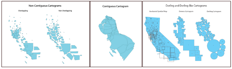
Fig. 4: Cartograms of population of the county map of California using (left) non-contiguous, (middle) contiguous, or (right) Dorling types. Image courtesy:
http://www.ncgia.ucsb.edu/projects/Cartogram_Central/types.html

^[2] Network data is represented using graph data structures. Nodes of a network correspond to vertices of graph, and links between nodes correspond to edges in the graph. We distinguish

 

3. Broadening the Scope of Geovisualizations

In this section, we discuss how geovisualizations can be constructed with abstract visual representations without the aid of cartographic maps. We have discussed about geovisualization exclusively for spatial data in Section 2. This can be extended to geospatiotemporal data, which is the type of data readily available today. Hence, the visualization of four-dimensional (4D) data is a relevant topic to discuss. Considering the prevalence of geospatial data with multiple attributes, we discuss some of the multivariate visual representations which are used in geovisualization.

3.1 Abstract Visual Representations

The visualizations discussed so far consider the maps in scale, which one can deviate from, when using Cartograms. Cartograms are graphics which map attribute properties to area of entities with boundaries, e.g. counties or districts, states, countries, etc. Though the Cartogram is generated from a cartographic map, it does not necessarily honor geographic precision, as demonstrated by its different types, in Figure 4.

Despite the presence of geo-reference data or metadata, not all geovisualizations are built with the reference of or in the context of a cartographic map, as shown by examples of metro map and volume visualization of geological models in Figure 5.
Abstractions such as schematic diagrams of transport networks and metro maps [18], serve purposes other than geo-references. In 1933, Harry Beck used “navigation through the London Underground” as a motivation for the design of the London Underground Map, popularly known as the Tube Map, today. Similarly, geological modeling and its visualization do not require the context of cartographic maps for understanding the geological processes. Visualizations of indoor of buildings or man-made habitations, e.g. for movement data in the building, can use abstractions based on floor plans. The floor plans may be considered to be maps, however, for most of the applications, they are used without geo-references. As an example, Lanir et al. [19] have used tangram diagrams to visualize the spatio-temporal behavior of museum visitors.

3.2 Geospatio-temporal Data Visualizations

While geospatial datasets pertain to two- or three-dimensional space, these datasets predominantly include temporal variations as well, making them geospatio-temporal datasets. Temporal aspects of the data are more effectively captured using animation in comparison to other techniques for visualization of four-dimensional (4D) datasets.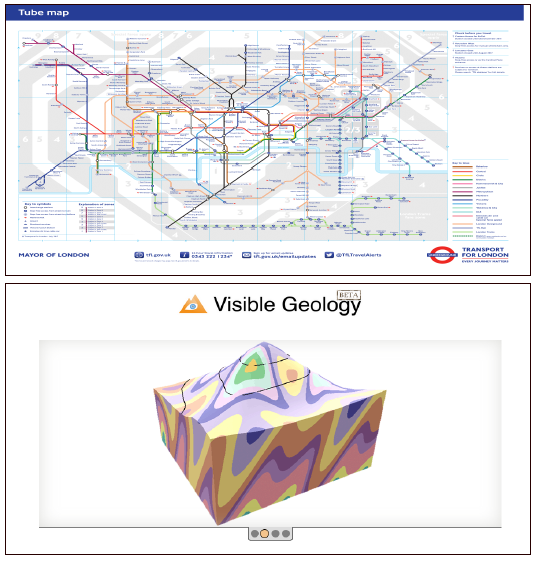

Fig. 5: Geovisualizations without the reference of cartographic maps. (Top) London Underground Map, or the Tube Map, is a schematic diagram which enables navigation through the London Underground system. (Bottom) Geological visualizations involve studying geometries or surface/volume topology involved in geology, such as folds, faults, etc.
(Image courtesy: https://tfl.gov.uk/maps/track/tube and http://app.visiblegeology.com/)

Adrienko et al. [2] have catalogued different methods used for exploratory analysis of spatio-temporal data. Their study maps different types of datasets and visualization tasks to corresponding types of geovisualizations and user interactions, for effective data analytics. For example, map animation is useful for time stepping for all types of data. However, specifically for existential changes (related to actual events) and location changes, space-time cube is used. A space-time cube is a 3D projection of the 4D data, where one spatial dimension, usually height, is not included. Space-time cubes are useful for tasks which do not require studying height changes; whereas, animation is the method to use for observing height changes, as it uses all of the 4D data.
With regard to map animation, Harrower and Fabrikant [12] have sensitized the need for application of appropriate design principles for dynamic (i.e. time-varying) visualizations. They have asserted the need for research in not just cartography, but also in animation and human cognitive science to make effective map animations. Map animations can be applied to all visualizations described so far. For example, understanding the mirror neuron system in neuroscience research helps in understanding the effectiveness of dynamic visualizations [35], as the mirror neuron system plays a key role in observational learning in motor tasks. A good example of map animation is the use of timelapse to demonstrate the changes on the Earth during 1984-2016, using the Google Earth Engine ³.

Bach et al. [3] have proposed the use of a generalized space-time cube data structure, which is the conceptual representation of time with respect to space. The visualizations are generated using different types of operations on the cube, which are effectively dimensionality reduction processes for converting three-dimensional cubes to readable two-dimensional visual representations. While the cube is applicable to geospatio-temporal data, its use can be extended to other datasets such as videos, networks, etc. The operations include space shifting, time flattening, time juxtaposing, etc., which may be a singleton or multiple operations. The humble origins of the term space-time cube comes from the definition of the term, “time geography” by Torsten Hägerstrand in 1970 [9], which is the “a time-space concept” for developing a kind of socio-economic web model.

3.3 Multivariate Geovisualization

Most GIS (geographic information science) datasets acquired today contain more than one variables. e.g. for study of land-use, one considers three categories of variables, namely, elevation, edaphic factors, and climatic factors, which altogether are nine variables [11]. The edaphic factors include plant-available water capacity, soil organic matter, etc.; and the climatic factors include mean precipitation, degree-day heat sum, etc. during growing season. Another example of such multivariate geospatio-temporal data is a household survey dataset for assessing public health programmes. Survey data has as many variables as the number of questions in the survey questionnaire [32].

between the usage of “vertices” and “edges” for the data structure, and “nodes” and “links” for the network data itself.
^[3] https://earthengine.google.com/timelapse/

The geovisualizations discussed so far, in their basic forms, represent one attribute, e.g., Cartograms are representations of a single attribute in the datasets. These representations become limiting for datasets with multiple attributes. To resolve this, one can additionally overlay cartographic maps or cartograms with glyphs having certain characteristics. Thus, one can visualize more variables using a composition of the aforementioned techniques.
Hargrove et al. [11] have shown how different color channels namely red, green, and blue, can correspond to three different variables and this multivariate heat map is used on map visualization. However, providing the spatial context for the visual representation of multiple attributes becomes a challenge at times. One of the strategies to circumvent this issue is the use of composite visualizations. Composite visualizations contain more than one visualizations which are to be used simultaneously. The taxonomy of composite visualizations [15] is based on the differences in the composition operator. The juxtaposed view is the most popular type of composite visualization, which is a juxtaposition of several visualizations. For multivariate geovisualizations, several single attribute map visualizations can be juxtaposed, an example of which is shown in [11], as well.
Another type of composite visualization is superimposed views. Geospace [23] is an example of overlaying different GIS layers, where each layer corresponds to an attribute or variable, and transparency is used to composite different layers, which is done to ensure that data in any layer is not inadvertently occluded.
Yet another example of composite visualizations is juxtaposing map-based visualizations with spatial-context-free multivariate visualizations, such that only the mapbased views preserve the spatial context. Popularly used multivariate visualizations are scatterplot matrices, parallel coordinates plot, and matrix visualization (Figure 6).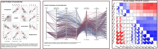

Fig. 6: Multivariate visualizations which can be juxtaposed with maps: (Left) scatterplot matrices, (middle) parallel coordinate plots, and (right) corrgram. These visualizations are for the multivariate automobile dataset, for demonstration purposes. Image courtesy:https://queue.acm.org/detail.cfm?id=1805128 [13] and http://www.infovis.info/index.php?words=exploratory
Scatterplot matrices lay out the scatter plots of pairwise variables in a matrix format. Each row of the matrix corresponds to a variable. The columns of the matrix correspond to the same set of variables, as the rows. The ordering of the variables in the rows and columns is the same. An element of the matrix is a scatterplot corresponding to the variables in the corresponding row and column of the matrix. A variant of the scatterplot matrix relevant for geovisualization is the one with embedded maps, called “multiform bivariate matrix with space fill and map” [25]. The idea here is to fill the upper triangular part of the matrix with maps, and lower triangular one with scatterplots. The upper triangular part gives the spatial context and the lower triangular shows overall correlation between variables taken pairwise.
Parallel coordinates plots (PCP) are used for identifying trends in overall data, as well as correlation between any two variables. Each of the parallel axes in the PCP corresponds to a single attribute or variable. A “polyline” in a PCP corresponds to a row in a table or log, and is an alternate representation to a point in the Cartesian coordinate plot. PCP is effective only if the axes can be swapped so that we can bring two axes together for correlation analysis.
Table or matrix visualization is a visual representation of the tabular or matrix format of the data where the variables and the entities (e.g. locations in geospatial data) are rows and columns, or vice versa. In the visualization, each matrix element is colored using a transfer function for the value represented in the element, thus giving a heatmap.
The matrix can be constructed in two different ways – two-way two-mode representation, and two-way one-mode representation. Two-mode representation is where the rows and columns represent different sets of objects. The one-mode representation implies that the same set of objects are used in both rows and columns, and their ordering is the same in both row and column. An example of the one-mode representation is the corrgram which is used for studying the correlation between two variables, given in the row and column. The corrgram additionally uses glyphs and color to indicate value and sign of the correlation. One-mode representation also includes association matrix (between variables) and similarity matrix (between objects). Matrix visualization is effective only if it allows the user to perform seriation or reordering of variables [21], which is a permutation of the ordering of variables. Seriation maintains the restriction that the ordering followed in rows as well as columns is the same permutation.
These visualizations are made effective with specific user interactions. Brushing and linking are relevant user interactions for parallel coordinates plot and scatterplot matrices. Brushing is equivalent to using a lasso to subselect a few set of points, and linking implies updating different visualizations based on highlighting the “brushed” sub selection. A rendering technique called edge bundling reduces the clutter of overlapping edges in the parallel coordinate plot.
There are other ways of encoding visualization channels (such as color, texture, geometry, etc.) with variables. Artistic rendering can also be used for multivariate visualization, e.g. in [34], where the painterly rendering styles, e.g. brush stroke length, brush thickness, etc. can be used to encode different variables, such that the final rendering shows the spatial trends in co-occurrences of different variables.
Reducing the complexity of multivariate data involves use of data mining algorithms. Jin et al. [16] have used multivariate clustering using self organizing maps (SOMs). Colors assigned based on clusters in SOM are used for choropleth map visualization. Inspired by the same methodology of multivariate clustering, Zhang et al. [36] compare clustering results using choropleth maps, parallel coordinates plot, rose plots, and scatter plots for principal component analysis (PCA). While these works are listed as geovisualizations, the use of data mining (SOMs, PCA, etc.) makes them geovisual analytics applications.

4. Geovisual Analytics: A Case Study

In this section, we discuss a case study of a set of applications of geovisual analytics for similar datasets. Geovisual analytics is governed by the nature of the dataset, its complexity, its analytical goals, and its stakeholders. Hence, we briefly explain these aspects of the two tools covered in the case study for analysis of transport networks.

4.1 Taxi Trajectories (Transport Networks)

We consider two visual analytics systems used for taxi trajectories, namely, VAIT [22] and TrajGraph [14]. VAIT is designed to be a scalable tool for statistical analysis, and TrajGraph for graph-based analysis. VAIT is targeted to improve the profits and productivity of the taxi services. TrajGraph is used for studying traffic congestion using taxi trajectory data.

VAIT is a visual analytics tool designed to analyze metropolitan transportation dataset for making sense of the data, and planning for efficient utilization. The data is acquired from vehicle Global Positioning Systems (GPS’s), and sensors deployed on the road banks. The test data in [22] is from 15,000 taxis running for two months in a city in China with population of 10 million. The data preprocessing step involves a novel calibration technique to account for missing or corrupt data owing to high vehicle mobility and variance in environment. Owing to the volume of the data, queries are made efficient by performing them on road segments, and then embedding taxi GPS data on the concerned road segments. To visualize trajectory of large number of taxis, the tool has been designed to use queries to reduce the data clutter, and improve caching to make visualizations responsive as well as make the system scalable. VAIT has been designed to solve 12 different predefined queries, e.g. finding at a given time, (Q1) the location or trajectory of given taxi at given time, (Q2) top n speeding taxis at a given time, (Q3) top n taxis by revenue, (Q4) origins and destinations of trips, (Q5) top n taxis by number of transactions or rides, etc.
After the execution of a novel weight-based calibration method, the visual display of movement data is captured using a novel visualization aided mining approach, called visual fingerprinting (VF). The visualizations are either trajectory or heatmap visualizations. In trajectory-style VF, the trajectory is rendered using B-splines, where the length of the trajectory gives the trip distance, and its color gives the number of visits to the destination location using average speed of each trip from source to destination. In the heatmap-style VF, one uses the index matrix constructed with number of taxi samples on the roads, average speed of these taxis, or the rank of number of passengers getting on/off at the location. The larger values imply “hotter” the map. A circle is used for encoding daily or monthly distribution of the taxis on the road.

The visual analytics process entails fingerprinting the entire dataset for an overview.

The cartographic map is used for display of statistical information, which gives leads on interesting locations to explore further. The overview also includes the traffic flow visualization. Subsequent to the overview, the users can drill down to specific road segments or locations and do further analysis. The spatial analysis is done using the heatmap, where the spatial distributions of the features are computed. This is then used for studying temporal trends. For temporal analysis, the visual fingerprints are associated with temporal information, e.g. time taken, average speed, frequency of passing taxis, etc. The temporal analysis is done for 24-hour time period over a week or a month. The hourly distribution is colored, and temporal and spatial changes are observed by comparing different fingerprints. VAIT system relies on the querying and filtering process after the global overview, for facilitating scalability. VAIT is one of the pioneering visual analytical system which is scalable and which embeds traffic flow results on spatio-temporal movement data.
TrajGraph is a visual analytics method which is integrated with graph modeling, for studying urban mobility using taxi trajectory data. A graph is used as a data structure to store and organize information of the taxi trajectory over city streets. Then a graph partitioning algorithm is run to split to regional-level subgraphs, as opposed to street-level subgraph. The visualizations include node-link diagram of the graph without map information, a map-based visualization (for symbols and trajectories), and a temporal data visualization. These three visualizations are composite using juxtaposed views, and are linked. There is a score of importance for different regions, which is computed using Pagerank and betweenness centralities of the graph. The graph partitioning provides different scales of the data, where the multi scale visualization includes city-wide graph, then region-level, and then street-level.
The centralities are compared across time, e.g. a location with high Pagerank but low betweenness indicates a frequently visited location but a weak connection to reaching other location. A segment with high betweenness may be perceived to be a fast bypass route, and its betweenness dropping during rush hours indicates it is less preferred during the rush hours. Similar to temporal analysis, the graph modeling allows spatial analysis using the local regional analysis. One can identify high traffic regions as locations with high Pagerank and high betweenness
centralities.
An urban transportation expert would use TrajGraph for troubleshooting traffic congestion. TrajGraph, a web-based prototype, opens the city-wide graph in the node-link graph view, and then shows betweenness centrality using color, for the 24-hour period. For road segments with high betweenness centrality, one can drill down further to see graph view and the map view. Given the map view, one can also drill down areas neighboring to problem areas. One can compare temporal variations in betweenness across different locations or regions, to understand their significance better. One can study variations leading to the rush hour traffic. One can identify urban traffic bottleneck, and study its pattern over a time period of time to confirm problem areas. One can then improve on the traffic congestion by resolving traffic flows during critical time-periods in these problem spots.

4.2 Broadening the Scope of Geovisual Analytics

As can be seen from Section 4.1, the design, implementation, and usage of the visual analytics solution depend heavily on the applications. At this juncture, we can add several research directions to the area of geovisual analytics. These research directions are significant in opening up research challenges and opportunities in pushing the area of geovisual analytics forward. We discuss two such research directions in this paper.
In the case study, we have discussed how introducing a data structure, such as graphs, or introducing a data preprocessing step, such as filtering, improves the visual analysis. Here, we discuss how we can integrate different domain-specific analyses which can improve on the visual analytics solution. The first research direction is on studying such amalgamations. We discuss further on one such amalgamation, namely, between spatial and social network analyses to give rise to geo-social network analysis. The second research direction is on user interfaces for geovisual analytics. An example of such a user interface is one with natural user interactions, that exploit the spatial context of the geospatio-temporal data. That would imply that one can use modes of human-computer interactions other than on a conventional personal computer, namely an immersive virtual reality.

Geo-social visual analytics has been studied by Luo and MacEachren [24], who have found that in social network analysis, spatial data is treated as background information and in geographical analysis, network analysis is oversimplified. Hence, they have argued for integrating knowledge from both analysis for datasets which have both geographic as well as social network data, e.g. location based social networks. They have called this integrated analytical approach as geo-social visual analytics. In their work, they have proposed the theoretical framework where the contexts can be brought together, and they have reviewed the state-of-the-art in the three core tasks for geo-social visual analytics, namely, exploration, decision making, and predictive analysis, to find gaps. They have used this gap analysis to identify potential challenges and research directions. Here, we discuss the authors’ views on the conceptual framework and the core tasks of data exploration and decision making.

• • The First Law of Geography says, “Everything is related to everything else, but near things are more related than distant things,” and the social network analysis dogma says, “Actors with similar relations may have similar attributes/behavior.” The authors have discussed how the First Law of Geography and the social network analysis dogma must be both combined to define geo-social relationships. At a conceptual level, these relationships are considered to be the intersection set of three different kinds of embeddedness. The different kinds of embeddedness are namely societal, network, and territorial. Thus, the conceptual framework for geo-social relationships states that “Nearness can be considered a matter of geographical and social network distance, relationship, and interaction.’

 

• • The core task of data exploration must consider the relative strength between the two aspects of the data. One of the aspects qualify geo-social relationships as being “among geographical areas” and the other, as being “among individuals at discrete locations.” While the visualizations generated are similar for both sets, for the latter,it requires additional computational processes for exploring the “spatial-social human interactions focus on developing quantitative representations of human movements.”

 

• For the core task of decision making, spatial data analyses exploit spatial locality to study trends, and relate them to explanatory covariates such as demographic data. Network analysis grows in a bottom-up fashion, whereas geographical analysis tends to be top-down. Integrating both can be done using linked methods where individually the visualization techniques cater to specific needs of both the analyses.

 

Some of the future research directions are towards:

(a) developing theory, methods, and tools, integrating the two separate aspects of the data;

(b) understanding the dynamics of geo-social relationships and processes;

(c) integrating ideas in cognitive sciences supporting geo-social visual analytics; and

(d) developing new geo-visual analytical methods for the three core tasks.
Virtual Reality for Geovisual Analytics has been studied by Moran [27], who have proposed that one could separate the preprocessing step of data modeling and analytics from the visualization processes. The visualization process can then be implemented in a virtual reality platform so that the user gets better situational awareness and can use natural user interactions for further analysis.
While the visual representations are approximately the same in immersive as well as non-immersive visualizations, we find that the user interactions for analytical tasks are improved in immersive geovisual analytics. The five tasks in the visualization workflow include navigation or exploration; identification and selection; querying and filtering; clustering; and details-on-demand. Navigation is achieved through fly-through cameras with change of perspectives, where the user can virtually navigate through the life size virtual model of the space. Depending on the approach of the user to objects in the scene, zooming can also be used.

Identification exploits the differences in rendering different geometric primitives for the visual representation of the data, e.g. shape and color can be used for “picking” features of interest. Filtering and querying can be provided using a virtual keyboard, and menu options in the Graphical User Interface (GUI). Clustering and pattern matching can be done by virtually overlaying or stacking different layers pertaining to the data, e.g. height of the data with population. Details-on-demand can be implemented using the levels of organizing data, and drilling down deeper as per requirement. In an immersive virtual reality, the user can a directed 3D arrow to enable direct interaction with the scene and enabling movement as required.
^[4] The age of the area of geovisualizations is not certain. There are references to visualization in paper as early as Philbrick (1953). This observation has been made by MacEachren and Kraak (1997).

The visual analytics solution in [27] relies on the current state-of-the-art in both geovisual analytics as well as virtual reality technologies. Much work is yet to be done here where it becomes the most preferred interface for the users for geovisual analytics. The separation of model from the user interactions may not be possible always. Hence, new strategies must be discovered for incorporating immersive characteristics throughout the data analytic workflow.

5. Road Ahead: Research Challenges

Geovisual analytics is the most recent successor in the evolution of visualization of geographic data, which had humble beginnings in cartography. Geovisualizations and geovisual analytics have matured in terms of methodologies and implementations across different types, complexities, and sizes of datasets, with geo-referencing. However, despite around 2 to 5 decades⁴ of work in geovisualizations, there remain multiple persistent challenges [7] in the area, which stem from gaps in:

(a) better understanding of scope of domain, how it interacts with other domains;
(b) a systematic understanding of human factors, e.g. cognitive, social, geographical, etc.; and
(c) a set of guidelines which can templatize the visualizations to data types, so that the practitioner is guided in designing appropriate and helpful visualizations corresponding to the tasks.
The reason for the persistence in these challenges is due to the interdisciplinary nature of the area of geovisualizations. As is the challenging with visualization in itself, evaluation or assessment of geovisualizations need work in future. These challenges have been documented by Keim et al. [17] too.
Ballatore et al. [5] have proposed the method for information search using spatial approaches. They argue for cross-fertilization of ideas between cognitive psychology, computer science and GIS to enable the use of spatial approaches. This cross-pollination is exactly the need of the hour for geovisualizations too [7]. Additionally, at the conceptual level, we find geovisualizations to be synonymous to spatial approaches for information search, by virtue of the inherent spatial nature of data.

In summary, we have provided a brief introduction to geovisualizaton, and how it is increasingly being resolved using geovisual analytics. We have discussed a sampling of the research challenge we often see in the area. The new advent in technology and more accessibility to datasets show promise in more innovations in this field.

Acknowledgements

 

The author is thankful to the members of the Graphics-Visualization-Computing Laboratory (GVCL) at the International Institute of Information Technology Bangalore (IIITB), both current and alumni, for inspiring the need for this article and developing body of work in geovisual analytics. The author is grateful to her colleagues at IIIT-B, and financial support for research in geovisual analytics from the Government of India, namely the Early Research Career Award from SERB, and other sponsored projects from DST, and INCOIS, and non-governmental organizations, such as Foundation for Research in Health Systems (FRHS), Bangalore.

References

[1]  Andrienko, G., Andrienko, N., Jankowski, P., Keim, D., Kraak, M.J., MacEachren, A., Wrobel,
S.: Geovisual analytics for spatial decision support: Setting the research agenda. International
Journal of Geographical Information Science 21(8), 839–857 (2007)

[2]  Andrienko, N., Andrienko, G., Gatalsky, P.: Exploratory spatio-temporal visualization: an
analytical review. Journal of Visual Languages & Computing 14(6), 503–541 (2003)

[3] Bach, B., Dragicevic, P., Archambault, D., Hurter, C., Carpendale, S.: A descriptive framework
for temporal data visualizations based on generalized space-time cubes. In: Computer
Graphics Forum. vol. 36, pp. 36–61. Wiley Online Library (2017)

[4] Badam, S.K., Elmqvist, N., Fekete, J.D.: Steering the craft: Ui elements and visualizations
for supporting progressive visual analytics. In: Computer Graphics Forum. vol. 36, pp. 491–
502. Wiley Online Library (2017)

[5] Ballatore, A., Kuhn, W., Hegarty, M., Parsons, E.: Special issue introduction: Spatial approaches
to information search (2016)

[6] Blumenfeld, J.: Getting Ready for NISAR – and for Managing Big Data using the Commercial
Cloud (December 2017), https://earthdata.nasa.gov/getting-ready-for-nisar, last accessed
on December 13, 2017

[7] Çöltekin, A., Bleisch, S., Andrienko, G., Dykes, J.: Persistent challenges in geovisualization–
a community perspective. International Journal of Cartography pp. 1–25 (2017)
[8] Fekete, J.D., Primet, R.: Progressive analytics: A computation paradigm for exploratory data
analysis. arXiv preprint arXiv:1607.05162 (2016)

[9] Hägerstraand, T.: What about people in regional science? Papers in regional science 24(1),
7–24 (1970)

[10] Hahmann, S., Burghardt, D.: How much information is geospatially referenced? networks
and cognition. International Journal of Geographical Information Science 27(6), 1171–1189
(2013)

[11]  Hargrove, W.W., Hoffman, F.M.: Potential of multivariate quantitative methods for delineation
and visualization of ecoregions. Environmental management 34(1), S39–S60 (2004)

[12] Harrower, M., Fabrikant, S.: The role of map animation for geographic visualization. Geographic
visualization: concepts, tools and applications pp. 49–65 (2008)

[13] Heer, J., Bostock, M., Ogievetsky, V.: A tour through the visualization zoo. Queue 8(5), 20
(2010)

[14] Huang, X., Zhao, Y., Ma, C., Yang, J., Ye, X., Zhang, C.: Trajgraph: A graph-based visual
analytics approach to studying urban network centralities using taxi trajectory data. IEEE
transactions on visualization and computer graphics 22(1), 160–169 (2016)

[15] Javed, W., Elmqvist, N.: Exploring the design space of composite visualization. In: Pacific
Visualization Symposium (PacificVis), 2012 IEEE. pp. 1–8. IEEE (2012)

[16] Jin, H., Guo, D.: Understanding climate change patterns with multivariate geovisualization.
In: Data MiningWorkshops, 2009. ICDMW’09. IEEE International Conference on. pp. 217–
222. IEEE (2009)

[17] Keim, D., Andrienko, G., Fekete, J.D., Gorg, C., Kohlhammer, J., Melançon, G.: Visual
analytics: Definition, process, and challenges. Lecture notes in computer science 4950, 154–
176 (2008)

[18] Kramer, J.: Is abstraction the key to computing? Communications of the ACM 50(4), 36–42
(2007)

[19] Lanir, J., Bak, P., Kuflik, T.: Visualizing proximity-based spatiotemporal behavior of museum
visitors using tangram diagrams. In: Computer Graphics Forum. vol. 33, pp. 261–270.
Wiley Online Library (2014)

[20] Li, S., Dragicevic, S., Castro, F.A., Sester, M., Winter, S., Coltekin, A., Pettit, C., Jiang, B.,
Haworth, J., Stein, A., et al.: Geospatial big data handling theory and methods: A review and
research challenges. ISPRS Journal of Photogrammetry and Remote Sensing 115, 119–133
(2016)

[21] Liiv, I.: Seriation and matrix reordering methods: An historical overview. Statistical Analysis
and Data Mining: The ASA Data Science Journal 3(2), 70–91 (2010)

[22] Liu, S., Pu, J., Luo, Q., Qu, H., Ni, L.M., Krishnan, R.: Vait: A visual analytics system for
metropolitan transportation. IEEE Transactions on Intelligent Transportation Systems 14(4),
1586–1596 (2013)

[23] Lokuge, I., Ishizaki, S.: Geospace: An interactive visualization system for exploring complex
information spaces. In: Proceedings of the SIGCHI conference on Human factors in
computing systems. pp. 409–414. ACM Press/Addison-Wesley Publishing Co. (1995)

[24] Luo, W., MacEachren, A.M.: Geo-social visual analytics. Journal of spatial information science
2014(8), 27–66 (2014)

[25] MacEachren, A.M., Gahegan, M., Pike, W., Brewer, I., Cai, G., Lengerich, E., Hardistry, F.:
Geovisualization for knowledge construction and decision support. IEEE computer graphics
and applications 24(1), 13–17 (2004)

[26] MacEachren, A.M., Kraak, M.J.: Research challenges in geovisualization. Cartography and
geographic information science 28(1), 3–12 (2001)

[27] Moran, A., Gadepally, V., Hubbell, M., Kepner, J.: Improving big data visual analytics with
interactive virtual reality. In: High Performance Extreme Computing Conference (HPEC),
2015 IEEE. pp. 1–6. IEEE (2015)

[28] Mulder, J.D., VanWijk, J.J., Van Liere, R.: A survey of computational steering environments.
Future generation computer systems 15(1), 119–129 (1999)

[29] Parker, S.G., Johnson, C.R.: Scirun: a scientific programming environment for computational
steering. In: Proceedings of the 1995 ACM/IEEE conference on Supercomputing. p. 52.
ACM (1995)

[30] Rosen, P.A., Hensley, S., Shaffer, S., Veilleux, L., Chakraborty, M., Misra, T., Bhan, R., Sagi,
V.R., Satish, R.: The nasa-isro sar mission-an international space partnership for science and
societal benefit. In: Radar Conference (RadarCon), 2015 IEEE. pp. 1610–1613. IEEE (2015)

[31] Schulz, H.J., Angelini, M., Santucci, G., Schumann, H.: An enhanced visualization process
model for incremental visualization. IEEE transactions on visualization and computer graphics
22(7), 1830–1842 (2016)

[32] Sreevalsan-Nair, J., Agarwal, S., Vangimalla, R.R., Ramesh, S., Murthy, N.: Collaborative
design of visual analytic techniques for survey data for community-based research in public
health. In: Proceedings of 8th Workshop of Visual Analytics in Healthcare (VAHC 2017).
pp. 1–2 (2017)

[33] Stolper, C.D., Perer, A., Gotz, D.: Progressive visual analytics: User-driven visual exploration
of in-progress analytics. IEEE Transactions on Visualization and Computer Graphics
20(12), 1653–1662 (2014)

[34] Tateosian, L., Amindarbari, R., Healey, C., Kosik, P., Enns, J.: The utility of beautiful visualizations.
In: Free and Open Source Software for Geospatial (FOSS4G) Conference Proceedings.
vol. 17, p. 18 (2017)

[35] Van Gog, T., Paas, F., Marcus, N., Ayres, P., Sweller, J.: The mirror neuron system and observational
learning: Implications for the effectiveness of dynamic visualizations. Educational
Psychology Review 21(1), 21–30 (2009)

[36] Zhang, Y., Luo, W., Mack, E.A., Maciejewski, R.: Visualizing the impact of geographical
variations on multivariate clustering. In: Computer Graphics Forum. vol. 35, pp. 101–110.
Wiley Online Library (2016)