We have all experienced a degree of frustration when a web page takes longer than expected to load. The delay between the moment when the user enters a URL (or clicks a link) and when the page contents are finally displayed has two causes: the time needed to fetch the page contents from one or more web servers (known as the end to end network delay) and the time needed to render the content in the browser window (known as the page load time). In this article, we will explore the components of the former delay via a simple set of experiments.

Introduction

In all types of interactions with computational devices, users have grown accustomed to rapid response times. In the context of web browsing, a delay of about one second is quite likely to result in the user mentally “context switching” to another task, while a delay of ten seconds may persuade the user to abandon the web page altogether [7]. This delay depends on the time for the network to transmit the page contents and the time for the browser to render these contents.

In this article, we will focus only on the first of these delays, known as the end to end network delay. This topic is described in popular computer network textbooks such as Peterson and Davie [4] (Section 1.5) and Forouzan [5] (Section 3.6). A more detailed explanation is given by Kurose and Ross [3], drawing on an analogy with a caravan of cars (corresponding to packets) traveling on a highway (link) with toll booths (switches) to illustrate the four sub-components of end to end delay, known as transmission delay, propagation delay, queuing delay and processing delay. We have found that our students find the following analogy more accessible.

Consider a group of N students who are asked to leave their classroom and attend a special lecture in the seminar hall in another building. Students then exit their classroom at a rate of R students per unit time and assemble as a group. The group walks the distance D to the seminar hall at a speed S. On the way, the group waits for M time units at the road crossing between classroom building and seminar hall on account of college vehicles travelling on the road. On reaching the seminar hall, the students take L time units to follow instructions to be able to hear the lecture. In this analogy, each student represents a single bit, and the entire group of N students represents a packet. The packet is transmitted from the source (the classroom) to the destination (the seminar hall) on a link (the path connecting their classroom to the seminar hall).

In this simplistic case, the transmission delay is the time for the entire packet (N students) to enter the link, which is N/R. The propagation delay is the time for the packet to travel the distance to the destination, which is D/S. The queuing delay is the time taken by which the packet is delayed on the way, which is M. Finally, the processing delay is the time for processing the entire packet, which is L. Hence, the end to end delay for the packet is:

This analogy can easily be made more complex, for instance by modeling switches, links with different transmission rates, multiple packets, etc. This pedagogical approach does appear to help students better understand each sub-component of end to end delay – we find that their performance on assessment items at the Familiarity level of mastery (as defined by the CS2013 reference curriculum defined by ACM-IEEE [1]) improves. However, students still struggle on assessment items aimed at higher levels of mastery (Usage and Assessment), such as questions that probe students on differences between these sub-components.
We believe that an experiential approach is essential for proper understanding of these concepts. In this article, we therefore describe a few experiments (consisting of a simple and minimal setup of two systems and one and/or two simple unmanaged switches), that enables readers to measure the individual sub-components of end to end delay, and compare these measurements with values predicted by the underlying theory. We have observed that students who compare measured vs. predicted values and think about causes of discrepancies (if any) gain a far better understanding of key ideas behind network delays, and display their mastery of these concepts in higher-order assessments.

Measuring Network Delays

Propagation delay corresponds to a time taken by a bit traversing on links from one end of the system to the other. If we assume that the speed S of electromagnetic/light waves in the link medium is constant, this delay depends purely upon (and is directly proportional to) the distance D (i.e., the total length of all links). This delay is only noticeable for satellite-based links (since communication satellites orbit about 36000 km above the earth’s surface.) It is miniscule in any local area network setup such as a college laboratory, or if the links are terrestrial (since D will be at most a few kilometers, whereas S will be close to the speed of light). Thus, we will assume that propagation delays are small enough to be ignored in our experiments.

Transmission delay is inversely proportional to the link bandwidth R (also called link speed) and directly proportional to the number of bits N in each packet. For dial-up links, R is typically 56kbps. For cellular 2G, R is of the order of a few kilobits per sec (kbps). For a 3G network, R varies from a few hundred kbps to 2Mbps. For a 4G network, R varies from 1Mbps to 20+ Mbps. Our experiments are based on Ethernet LAN, where R depends on the type of Ethernet: 10Mbps (Ethernet), 100Mbps (fast Ethernet) or 1000Mbps (Gigabit Ethernet). We will fix R in our experiments, and we will observe how the transmission delay changes as N changes.

Processing delay is the total time taken by every network element process and forward a data packet to the next device in the path, or to an application on the end system. In a network switch, for instance, the processing delay for a packet is the time taken by the switch to decide the outgoing interface on which this packet needs to be forwarded. This will involve processing the packet by extracting the destination address (IP or MAC), matching it with the switch’s forwarding table, and then determining the outgoing interface. Thus, this delay clearly depends on the compute power of each network element. For our experiments, we will introduce artificial delays of varying durations to simulate variations in compute power.

Queuing delay is the total time spent by a packet waiting in buffers of network elements (switches or routers) to get transmitted. This delay depends on the number of packets already in queue buffers of individual network elements, and on the queuing policy that each such element implements. Since the number of packets that are waiting will vary dynamically as per the network traffic, this delay can only be predicted accurately if the experimental setup is controlled and its traffic characteristics are known so that an appropriate queuing model can be applied.

Below we define few experiments that a reader should to do measure these delay components and compare these with observed values to develop a better understanding. At times, the measured values will differ from computed values and reader should develop a reasoning for the difference.

Experiment 1: Transmission Delay

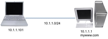
For this experiment, two machines (e.g., two desktops or laptops) are connected directly on an Ethernet LAN, as shown in Figure. 1. By default, laptop/desktop network interfaces are configured with DHCP protocol. Since there is no DHCP server here, configure these addresses manually (i.e., assign static IP Addresses).

To measure the network delay, we will send request packets from one machine to another, and receive the response packets (which is echo back of the request packet). The time elapsed will correspond to twice the end to end network delay. For our experiment, we will send five ping (ICMP) packets of various sizes between the two machines. In the terminal window of one of the machines, enter this command:
ping –c 5 –s N IP

Table-1: Response time between two directly connected hosts on a 10 Mbps Ethernet

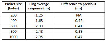
Using basic concepts discussed earlier, the theoretical transmission delay for N = 200×2 bytes (i.e., 400×8 bits) with R = 10Mbps (i.e., 107 bits per second) is seconds, or 0.32 ms.

Let us now compare this with the experimental data. Note that the times shown in Table-1 include all four sub-components of end to end delay, although propagation and queuing delays are negligible in this setup. The key for students is to realize that increasing packet sizes primarily increases only the transmission delay. Thus, the transmission delay for 200×2 byte packets can be estimated by computing the difference between successive rows in Table-1 (as shown in the final column). The difference between the observed value 0.42 ms and the computed value 0.32 ms can be attributed partly to measurement error and partly to the slightly different processing delays. The reader should note that the Ethernet link has a maximum packet size of 1500 bytes (MTU- Message Transmission Unit).
Thus, increasing the ping packet size beyond 1500 bytes would result in a ping packet getting split into multiple ethernet packets at the transmitting machine and joined at receiving machine. This is likely to add greater noise in the experimental measurements, but reader is encouraged to explore this option after the basic understanding is developed. This experiment makes it easy for reader to understand that transmission delay is directly related to packet size when the link bandwidth is fixed. By repeating this experiment with a bandwidth of 100 Mbps, students can grasp the relationship between transmission delay, packet size and link bandwidth.
As an extension to this experiment, add one network element, such as a simple Ethernet switch (4-port or higher) between the two machines, and again measure the response time for pings. By adding a network switch, the end to end delay will correspond to 4 links: Machine 1 to Switch, Switch to Machine 2, Machine 2 to Switch, and Switch to Machine 1. The result of our set of experiments with one intermediate switch added to the setup in Figure 1 is shown in Table-2.

Table-2: Response time between two hosts connected on a 10 Mbps Ethernet via a switch

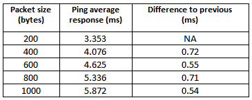
Let us understand this increased transmission delay. The intermediate Ethernet switch works in a store-and-forward mode i.e., it forwards a packet onto the next link only after it receives the entire packet. Hence, each link contributes to the overall transmission delay. The transmission delay for 200 byte packets corresponding to 4 links would be 0.64 ms (twice the 0.32 ms delay computed earlier, if we assume that a host sends only one packet at a time to the other host). The values of 0.55 ms and 0.54 ms in third and fifth rows are likely to be attributed to measurement errors. The average of these 4 values is 0.63 ms, which is very close to the theoretical expectation. The reader is recommended to conduct the experiment multiple times with different packet sizes (less than 1500 bytes).

Experiment 2: Processing Delay

To understand processing delay, we use our own client and server programs (instead of ping) for data communication. This ensures that data is handled at the application level, where processing delay can be introduced in a controlled manner. The key part of python code (using UDP protocol [2]) for a sample client application, running on Machine 1 and a server application running on Machine 2 is given in Appendix I. To simulate computation, the server application sleeps for a specified time tsleep. (In an actual application, this time would be spent on some meaningful action depending on the business logic, such as interacting with a payment gateway or querying a database server) The client sends several packets (e.g., 1000) and computes the delay in response.
The reader can observe how the delay varies with changes to tsleep. In our experiments, using the setup of two machines (connected via one switch) we observed the response time to be 3.22 ms when tsleep = 0 ms, and 13.23 ms when tsleep = 10 ms. The difference of 10.01 ms is the difference in processing delay of two packets. The reader is recommended to use Wireshark capture [6] on the server to look at the time when the client packet is received, and when the response is transmitted by the server. The Wireshark capture at the client will provide insights into the end to end network delay, because the time difference between a response packet and a request packet will include propagation and transmission delay (for all the links).

Experiment 3: Queuing Delay

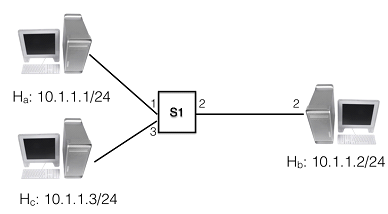
Within a network element, queuing delay can occur at three places: (1) at the input interface, where a packet is waiting to be received, (2) when packets wait in the buffer where the application needs to process it, and (3) at the output interface where it is waiting to be transmitted (the output interface can be busy transmitting other packets ahead in the queue). For queuing delay to occur, there must be at least two transmitters. (When two packets are being transmitted concurrently, one of them needs to wait.) We thus modify the setup for Experiment 1, with two or more clients sending data concurrently to the server. Two hosts Ha and Hc are connected to Hb via a single Ethernet switch on a 10 Mbps link ( Figure.2).

When two data packets are transmitted simultaneously from the two client machines, they will be queued at the input network buffer of the network switch, and at the input buffer of the server application until the server reads this data. It is practically very challenging to witness queuing at the switch since it will require very tightly coupled synchronization between the two client machines. (Even slight differences between two transmissions may not cause any queuing.) Thus, for simplicity, we will assume that all queuing delay occurs at the application input buffer.

The client machine sends the first packet, and then sends subsequent packets immediately after receiving a response for the previous packet. Since a client sends only one packet at a time, and sends the next one only after the response for the previous packet is received, there is no queuing delay at the client side.

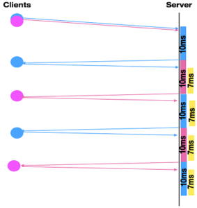
The simple server application is designed as single threaded – it reads data from the client, and it responds after sleeping for time tsleep (to emulate processing time delay). Once the response is sent, it immediately reads data from the next client request, processes it and responds back, etc. With a value of tsleep = 10 ms, the average response time is measured as 13.23ms. The end to end delay without any queuing is about 3.2 ms. With two clients, we observed response times of 20.21 ms and 20.22 ms measured by Ha and Hc respectively (with tsleep = 10 ms). Hence the queuing delay each packet encountered was about 7 ms (the difference between 20.21 ms and 13.23 ms). The delay of 7 ms can be explained in a simplistic way as follows. The delay of 3.23 ms for propagation, transmission and processing is subsumed in the queuing delay of 10ms at the application. Thus, each the packet needs to wait only for about 7 ms in the queue (not 10 ms).  The response time of 20.2 ms can be accounted as 3.2 ms of propagation and transmission delay, 10 ms of processing delay and 7 ms of queuing delay.
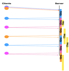
The reader is encouraged to conduct the experiment with three concurrent clients. Here, when a packet is being processed (for 10ms on account of tsleep = 10 ms), the request from the second client will wait for 7 ms, but the request from the third client will wait for 17 ms. Hereafter, all subsequent requests from all the three clients will witness a queue delay of 17 ms. Thus, the average response time for the clients is expected to be around 30 ms (corresponding to 17 ms for queuing delay, 10 ms for processing delay and 3 ms for propagation and transmission delay). Figure 3 and Figure 4 depict the processing and waiting (queuing) time for two and three concurrent clients respectively. The reader is encouraged to conduct experiments with four of more concurrent clients and analyze the queue delay and overall response time.

The reader is encouraged to modify the parameter tsleep, and notice that queuing delays are observed only when tsleep is substantially more than the transmission delay. If the value of tsleep is less than 3ms, there would be no queuing delays for second client.

The reader is further encouraged to conduct the experiment while keeping the processing delay smaller than the combination of transmission and propagation delays, and then observe and analyze the end to end delay. This would provide useful insights into interplay of these delays.
The importance of such experiments is valuable in the context of real-life applications which typically receive large numbers of concurrent requests. If application load causes significant delays, it is necessary to quantify the queuing delay and determine the causes of the processing delay, and then formulate strategies required to reduce the delay. We explore this issue in our next experiment. 

Experiment 4

This is an experiment to understand the impact of queuing and processing delays. The setup is identical to Experiment 3, but now the server application on Hb can spawn multiple server processes. To minimize noise in the timing measurements, these processes are pre-spawned by the server application, before it receives any client requests. Thus, there is no processing overhead of spawning child processes, which can vary depending upon the machine status. In our setup, the server application spawns three child processes, and thus the server can handle three concurrent client requests.

The reader should now replicate the earlier experiment with tsleep = 10 ms, and start the three concurrent clients. The average response time for each client program drops from about 20 ms to about 13.2 ms since the server’s CPU is free to handle each client’s request using separate processes. There is no queuing delay as each client request is processed by a separate application process.
We note that if the processing delay was due to CPU-bound computation on the server, the above strategy may exacerbate the delay especially on a single core CPU. For a multi core CPU system, as long as the number of server applications is less than number of CPU cores and each server process is assigned a different core, processing delay of one server application will not impact the processing by other server application. However, when processing delay of application is higher and leads to queuing of request, a different approach would be necessary, such as improving the algorithmic efficiency of the computation, using additional servers, etc.

Concluding Remarks

The end-of-semester feedback given by students on this experiential learning approach has been very encouraging. The students taught using this approach have fared much better, both in getting better jobs as well as later in professional life. A large number of them have said this has kindled their interest in the field of networking. Prior to this approach, students used to find the subject dry and difficult to understand.

Appendix I

Partial sample code of client and server program for experiments.

Client program code sample:

import socket
import time

sock = socket.socket(socket.AF_INET,
socket.SOCK_DGRAM)
srvr_addr = (‘10.1.1.1’, 9997)

sum = 0.0
for i in range(1,1000):
start_time = time.time()
sent = sock.sendto(msg, srvr_addr)
data, server = sock.recvfrom(4096)
end_time = time.time()
sum = sum + end_time – start_time

#compute resp time for one request
resp_time = sum / 1000

print “Resp time = “, resp_time

Server program code sample:


import socket
import time

sock = socket.socket(socket.AF_INET, socket.SOCK_DGRAM)
server_address = (‘10.1.1.1’, 9997)
sock.bind(server_address)

while True:
data, addr = sock.recvfrom(2000)
if data:
time.sleep(.010) #srv proc time
sent = sock.sendto(data, addr)

References

[1] ACM/IEEE Computer Society, “Computer Science Curricula 2013: Curriculum Guidelines for Undergraduate Degree Programs in Computer Science”, Joint Task Force on Computing Curricula, Association for Computing Machinery (ACM) and IEEE Computer Society, ACM, New York, NY, 2013.

[2] RFC 768, “User Datagram Protocol (UDP),”, Request for Comments 768. John Postel, ISI, August 1980.

[3] Kurose, Ross, “Computer Networks: A Top Down Approach” 7th edition, Pearson Education Inc, 2016.

[4] Peterson, Davie, “Computer Networks: A Systems Approach” 5th edition, Morgan Kaufmann, 2012.

[5] Forouzan, “Data Communications and Networking”, 4th edition, The McGraw-Hill, 2011.

[6] Wireshark: https://www.wireshark.org,  Last accessed 2017-11-30.

[7] Grigorik, “High Performance Browser Networking, Chapter 10”, O’Reilly, 2014.