A QUARTERLY PUBLICATION OF ACCS
Automotive Radars


Sujeet Patole
Murat Torlak
Dan Wang
Murtaza Ali

© 2017 IEEE. Reprinted, with permission, from IEEE Signal Processing Magazine, March 2017 
Automotive radars, along with other sensors such as lidar, (which stands for “light detection and ranging”), ultrasound, and cameras, form the backbone of self-driving cars and advanced driver assistant systems (ADASs). These technological advancements are enabled by extremely complex systems with a long signal processing path from radars/sensors to the controller. Automotive radar systems are responsible for the detection of objects and obstacles, their position, and speed relative to the vehicle. The development of signal processing techniques along with progress in the millimeter- wave (mm-wave) semiconductor technology plays a key role in automotive radar systems. Various signal processing techniques have been developed to provide better resolution and estimation performance in all measurement dimensions: range, azimuth-elevation angles, and velocity of the targets surrounding the vehicles. This article summarizes various aspects of automotive radar signal processing techniques, including waveform design, possible radar architectures, estimation algorithms, implementation complexity-resolution trade-off, and adaptive processing for complex environments, as well as unique problems associated with automotive radars such as pedestrian detection. We believe that this review article will combine the several contributions scattered in the literature to serve as a primary starting point to new researchers and to give a bird’s-eye view to the existing research community.


Introduction

 
The history of radio detection and ranging, more commonly known as radar, starts with the experiments carried out by Hertz and Hülsmeyer on the reflections of electromagnetic (EM) waves and ideas advocated by Tesla and Marconi in the late 19th and early 20th centuries. Earlier developments in radar technology were limited to military applications such as aircraft/ship surveillance, navigation, and weapons guidance. Radar is now used in many applications, including civilian aviation, navigation, mapping, meteorology, radio astronomy, and medicine. The main objectives of a radar system are to detect the presence of one or more targets of interest and estimate their range, angle, and motions relative to the radar [1].

To the everyday person, tangible applications of radar include speed guns used by law enforcement officers to detect speeding drivers. Action heroes in movies sometimes drive a fancy car with attractive features that can track an enemy’s speed and location, move swiftly and automatically amid obstacles, and debut its night vision feature during the movie’s climax. The ambition of having all of these add-ons to a car has become feasible with the flourishing mm-wave circuit technology and advanced signal processing techniques. Advances in circuit technology reinforced by new signal processing algorithms, machine learning, artificial intelligence, and computervision techniques have made self-driving cars a reality.

Advances in circuit technology reinforced by new signal processing algorithms, machine learning, artificial intelligence, and computervision techniques have made self-driving cars a reality.

Such cars also rely on different sensors such as a laser, a camera, ultrasound, global positioning system, and radar. Among these sensors, radar offers the possibility of seeing long distances ahead of the car in poor visibility conditions, which can help avoid collisions [2]. For example, Google’s self-driving car [3] has radars mounted on both front and rear bumpers of the vehicle to detect objects in its surroundings.

Automotive radars were first deployed several decades ago. The evolution of automotive radar from its inception to the present has been thoroughly discussed in [4]. With highly integrated and inexpensive mm-wave circuits implemented in silicon, compact automotive radar safety systems have become a popular feature [5][6]. Since then, review articles written on automotive radar mostly covered the circuit implementation, market analysis, and architectural-level signal processing [7] [8] [9]. However, there are many aspects of automotive radar signal processing techniques scattered throughout the literature. For example, a part of the literature may concentrate on detecting the presence or absence of targets, while another might look at radar estimation problems concerning their location and velocity in space relative to the radar [10][11]. This article’s goal is to review principal developments in signal processing techniques applied to estimating significant target parameters such as range, velocity, and direction. The article also discusses the characterization of radar waveforms and advanced estimation techniques that enhance the operation of automotive radars. In particular, we review each topic with adequate mathematical framework so as to make this a good start-up document for the newcomer in the field.

Automotive radar classification

 
Both autonomous and human-driven cars are increasingly using radars to improve drivers’ comfort and safety. For instance, park assist and adaptive cruise control provide comfort, while warning the driver of imminent collisions and overriding control of the vehicle to avoid accidents improve the safety. Figure 1 depicts various such radar subsystems that form ADASs. Each subsystem has unique functionality and specific requirements in terms of radar range and angular measurement capability (Table 1). The next section explains the fundamentals of location and speed estimation using the radar measurements.

Basic automotive radar estimation problems

 
A radar can simultaneously transmit and receive EM waves in frequency bands ranging from 3 MHz to 300 GHz. It is designed to extract information [i.e., location, range, velocity and radar cross section (RCS)] about targets using the EM waves reflected from those targets. Automotive radar systems typically operate at bands in 24 GHz and 77 GHz portions of the EM spectrum known as mm-wave frequencies so that higher velocity and range resolution can be achieved. Fundamental radar operation involves three main tasks: range (distance), relative velocity, and direction estimation, as discussed next.


Range estimation

 
The range estimation is fundamental to automotive radars. The range R, to a target, is determined based on the round-trip time delay that the EM waves take to propagate to and from that target: R = (cτ/2), where τ is the round-trip time delay in seconds and c is the speed of light in meters per second (c = 3 X 10⁸ m/s). Thus, the estimation of x enables the range measurement [1]. The form of the EM waves (signals) that a radar transmits is important for round-trip time delay estimation. For example, pulse-modulated continuous waves (CWs) consist of periodic and short power pulses and silent periods. Silent periods allow the radar to receive the reflected signals and serve as timing marks for radar to perform range estimation as illustrated in Figure 2. However, unmodulated CW signals (i.e., Cos(2πfct)) cannot be used for range estimation since they lack such timing marks. Additionally, the signal reflected from a target should arrive before the next pulse starts. Hence, the maximum detectable range of a radar depends on pulse repetition interval TPRF. The transmitted signal from the radar until it is received back undergoes attenuation due to the path loss and imperfect reflection from the target. In addition, received target signals are subject to internal noise in radar electronics and interference that may be a result of reflected signals from objects not of interest and may come from human-made sources (i.e., jamming). The typical round-trip time delay estimation problem considers only ambient noise in the form of additive white Gaussian random process. It is assumed that demodulation has already removed the carrier so that a target signal x(t) at baseband can be modeled as

where α is a complex scalar whose magnitude represents attenuation due to antenna gain, path loss, and the RCS of the target and w(t) is additive white Gaussian noise with zero mean and variance σ2. The goal is to estimate τ with the complete knowledge of the transmitted radar waveform s(t). Assuming the signal s(t) has unit amplitude and finite energy Es, the ideal radar receiver can be found using a matched filter with the impulse response h(t) = s*(-t), which maximizes signal to noise ratio (SNR =(α2Es2) =(α2Ts2) at the output. Thus, the matched filter-based receiver finds the correlation between the transmitted signal and received reflected pulses

The maximum likelihood (ML) estimate of the time delay is the time that the magnitude of the matched filter output peaks at

equation 3

The presence of the noise can perturb the location of the peak, which will result in the estimation error. Furthermore, the radar needs to decide whether or not a received signal actually contains an echo signal from a target. A good deal of classical radar literature is devoted to developing strategies that provide the most favorable detection performance.

A typical decision strategy can be formulated based on statistical hypothesis testing (a target present or not). This leads to a simple threshold testing at the matched filter output. Range resolution, another key performance measure, denotes the ability to distinguish closely spaced targets. Two targets can be separated in the range domain only if they produce nonoverlapping returns in the time domain. Hence, the range resolution is proportional to the pulsewidth Tp . In other words, finer pulses provide higher resolution. However, shorter pulses contain less energy, which implies poor receiver signalto- noise ratio (SNR) and detection performance. As explained in the section “Radar Waveforms,” this problem is overcome by the technique called pulse compression, which uses phase or frequency modulated pulses.

Velocity estimation

 
Estimation of the target velocity is based on the phenomenon called the Doppler effect. Suppose the car displayed in Figure 2 is moving ahead with differential velocity v. With the existence of relative motion between two cars, the reflected waves are delayed by time τ =(2(R±vt)/c). The time dependent delay term causes a frequency shift in the received wave known as the Doppler shift fd =(±2v/λ). The Doppler shift is inversely proportional to wavelength λ, and its sign is positive or negative, depending on whether the target is approaching or moving away from the radar. While this frequency shift can be detected using CW radar, it lacks the ability to measure the targets range. Here, we discuss a pulsed radar configuration that uses frequency modulated (FM) CW pulses and provides simultaneous range velocity estimation in multitarget traffic scenarios.

The FMCW radar transmits periodic wideband FM pulses, whose angular frequency increases linearly during the pulse.

For the carrier frequency, fc and FM modulation constant K, a single FMCW pulse can be written as [see Figure 3(a)]

The signal reflected from a target is conjugately mixed with the transmitted signal to produce a low-frequency beat signal, whose frequency gives the range of the target. This operation is repeated for P consecutive pulses. Two-dimensional (2-D) waveforms in Figure 3(c) depict successive reflected pulses arranged across two time indices. The slow time index p simply corresponds to pulse number. On the other hand, the fast time index n assumes that for each pulse, the corresponding continuous beat signal is sampled with frequency fs to collect N samples within the time duration T. Assuming single target and neglecting reflected signal distortions, the FMCW radar receiver output as a function of these two time indices is given by

Therefore, as illustrated in Figure 3(c), discrete Fourier transform across fast time n can be applied to obtain beat frequency fb =(2KR/c) coupled with Doppler frequency fd . This operation is also known as the range transform or range gating, which allows the estimation of Doppler shift corresponding to unique range gate by the application of second Fourier transform across the slow time. A range-Doppler map can be found efficiently by using 2-D fast Fourier transform (FFT) (5). A demonstrative example based on the aforementioned discussion is shown in Figure 3.


Direction estimation

 
Use of wideband pulses such as FMCW provides discrimination of targets in both distance and velocity. The discrimination in direction can be made by means of an antenna array. Figure 4(a) depicts a realistic traffic scenario with several targets surrounding the radar that collects direct and multipath reflections from them. In such cases, to spatially resolve equidistant targets and deliver a comprehensive representation of the traffic scene, the angular location of targets should be estimated. Therefore, in automotive radars, the location of a target is often described in terms of a spherical coordinate system (R,θ,∅), where (θ,∅) denote azimuthal and elevation angles, respectively. However, in this case, the single antenna radar setup as used in the range-velocity estimation problems may not be sufficient, since the measured time delay τ =(2(R±vt)/c) lacks the information in terms of angular locations of the targets.

To enable direction estimation, the radar should collect reflected wave data across multiple distinct dimensions. For example, locating a target using EM waves in 2-D requires the reflected wave data from the object to be collected in two distinct dimensions. These distinct dimensions can be formed in many ways using combinations of time, frequency, and space. For instance, a linear antenna array and wideband waveforms such as FMCW form two unique dimensions [13][14]. Additionally, smaller wavelengths in mm-wave bands correspond to smaller aperture sizes and, thus, many antenna elements can be densely packed into an antenna array. Hence, the effective radiation beam, which is stronger and sharper, in turn, increases the resolution of angular measurements.
 
Consider an antenna array located in plane z = 0, and let l be the abscissa corresponding to each receiver antenna position [see Figure 4(b)]. Let (Rq,iq) be the position of the qth target in spherical coordinates, moving with velocity vq relative to the radar. With the help of far-field approximation [15], for the qth target, the round-trip time delay between a transmitter located at the origin and the receiver positioned at coordinate l is given by

where d is the distance between antenna elements (usually half the wavelength) arranged in a linear constellation. Combining (5) and (6) gives the three-dimensional (3-D) FMCW radar output signal, which enables estimation of range, velocity, and angle. For Q number of targets, the signal can be represented as

where α and ω correspond to same quantities as explained in the range estimation problem. The delay term τlq creates uniform phase progression across antenna elements, which permits the estimation of the angle by FFT in the spatial domain, as shown in (7). Thus, 2-D location (range and angle) and speed of targets can be jointly estimated by 3-D FFT. The target location and velocity estimation problems are revisited later in the section “Advanced Estimation Techniques” with more emphasis on the high-resolution algorithms and computational complexity analysis.

Radar waveforms

 
Various automotive radar classes, summarized in Table 1, have diverse specifications in terms of several fundamental radar system performance metrics, such as range resolution, velocity resolution, angular direction, SNR, and the probability of target detection. The type of waveform employed by a radar is a major factor that affects these metrics. The radar waveforms, as summarized in Table 2, can be characterized whether or not they are CW, pulsed and frequency, or phase modulated. Modulated radar waveforms include FM CW, stepped frequency (SF) CW, orthogonal frequency-division multiplexing (OFDM), and frequency shift keying (FSK). Each waveform type has a certain advantage in processing, implementation, and performance as follows:

    • In the CW radar, a conjugate mixing of a high-frequency transmitted and received signal produces the output signal at the Doppler frequency of the target. The resolution of frequency measurement is inversely proportional to the time duration of the signal capture. The continuous nature of the waveform precludes round-trip delay measurement, which is necessary for range estimation of the target [see Figure 5(a)]. Hence, apart from ease of implementation and ability to detect target speed, the CW radar cannot provide the range information.
    • Pulsed CW radar can estimate the range information as explained previously in the section “Basic Automotive Radar Estimation Problems.” The Doppler frequency can be estimated by making each pulse longer and measuring the frequency difference between the transmitted and received pulses. As shown in Figure 5(b), the pulse duration and pulse repetition frequency (PRF) are the key parameters in designing pulsed CW radar with desired range and velocity resolution.
    • FMCW, also known as linear frequency modulation (LFM) or chirp, is used for simultaneous range and velocity estimation (refer to the “Velocity Estimation” section for details). Due to the pulse compression, the range resolution is inversely proportional to the bandwidth of the FMCW signal and is independent of pulsewidth. For example, the short-range FMCW radar uses ultrawideband (UWB) waveforms to measure small distances with higher resolution. The Doppler resolution is a function of pulse width and the number of pulses used for the estimation. Thus, with the ability to measure both range and speed with high resolution, FMCW radar is widely used in the automotive industry.

The traffic imaging problem can be turned into a classical parameter estimation problem so that superresolution techniques such as MUSIC can be applied.

  • In contrast to FMCW waveforms, the frequency of FSK and SFCW varies in a discrete manner [see Figure 5(c)]. In this case, the range profile of the target and the data collected at discrete frequencies form the inverse Fourier transform relationship. Also, hybrid waveform types can be employed to achieve additive performance. FSK waveform can be combined with multislope FMCW waveform to overcome ghost targets in radar processing [16]. Similarly, alternate pulses of CW and FMCW are used to accurately estimate range and Doppler [17].
  • OFDM can be viewed as another multifrequency waveform that offers unique features of the joint implementation of automotive radar and vehicle-to-vehicle communications [18][19]. For the radar operation, the orthogonality between OFDM subcarriers is ensured by choosing carrier spacing more than maximum Doppler shift, and the cyclic prefix duration is selected greater than the longest round-trip delay [see Figure 5(d)]. The range profile is estimated through frequency domain channel estimation. OFDM radar processing along with simulation results is explained in [20].

Based on the knowledge of target statistics, radar waveforms can be optimized. Radar waveform design is revisited along with multiple-input, multiple-output (MIMO) radars in the “MIMO Radar” section. 

Advanced estimation techniques

 
Advancements in silicon semiconductor technology have had the profound impact on the design of automotive radar systems, providing higher integration and performance at lower cost. This section reviews some sophisticated radar signal processing algorithms, which have become feasible with such advancements, especially for real-time implementation. In this section, most commonly used FMCW radar architecture is assumed and targets are considered to be stationary. Hence, (7) is reduced to a range-azimuth estimation problem with the signal model given by

To elucidate advanced estimation techniques, the dimensionality of the problem is reduced to two dimensions. It should be noted that the discussed techniques can be extended to four-dimensional problems with mobile targets and elevation direction. As discussed previously, the 2-D FFT of (8) can provide joint estimation of distance and angle. The FFT-based estimation has the least complexity of implementation, which is O(LN log LN), where N is the number of time domain samples and L denotes the number of elements in a one-dimensional (1-D) antenna array. However, the resolution of Fourier techniques is dictated by the Rayleigh limit. While the higher range resolution can be obtained with larger FMCW bandwidth, the higher angular resolution requires more antenna elements, adding to the cost of RF front end. Additionally, the radar has to process a larger set of signal samples. However, it is important to reduce the computational load while realizing the desired angular and range resolution. We first visit the ML formulation of joint estimation of range and direction of targets. Then, we review the so-called superresolution techniques as suboptimal and lower complexity alternatives to the ML estimator.

ML estimation

 
The complex Gaussian observation noise in (8) is assumed to be temporally and spatially independent. ML estimation of 2-D parameters (R,θ) can be found solving the following equation:

Thus, depending on the granularity of (R,θ) search space, the ML estimator can offer the resolution beyond the Rayleigh limit set by system parameters such as bandwidth and number of antenna elements. However, the complexity of implementing this algorithm depends on the cardinality of the search-space as well as the number of targets. Since (Rq,iq) are continuous parameters, the computational complexity of ML algorithm O(|(R, θ)|Q) becomes prohibitive. In the subsequent paragraphs, the superresolution techniques that can achieve high resolution at lower computational cost are illustrated.

Superresolution techniques

 
Due to their prohibitive computational cost, ML algorithms need to be implemented via suboptimal techniques. These techniques rely on collecting enough signal samples. At a sufficiently high SNR, eigenvalues and associated eigenvectors of sample covariance matrix C (defined in Algorithm 1) represent the ML estimate of their true values. Hence, these eigenvectors can be used to resolve the target with high resolution.

The superresolution algorithms that rely on these techniques include multiple signal classification (MUSIC) [24] and estimation of signal parameters via rotational invariance technique (ESPRIT) [25][26]. Recalling the 2-D (R,θ) stationary target location estimation problem, the superresolution algorithms can be applied across each dimension separately. However, this approach might lead to the so-called association problem [15]. Since the association of estimated parameters is the key step in interpreting and delivering results to the driver assist system, joint processing can be implemented. As (R,θ) domain is jointly searched for its entire range, the possibility of ghost targets is eliminated and unambiguous results are obtained [27].

For proper transmitter spacing, the colocated MIMO radar can emulate a larger aperture phased array radar.

As discussed previously, the temporal frequency of (8) gives the range, and spatial frequency corresponds to the angular position of the target. Hence, the traffic imaging problem can be turned into a classical parameter estimation problem so that superresolution techniques such as MUSIC can be applied. From (8), a 2-D matrix is formed, which has a Vandermonde structure across each dimension for a uniform linear antenna array. A 2-D joint superresolution was applied in the radar imaging context in [27] and later with FMCW waveforms in [21], which is described in Figure 6 and Algorithm 1. The complexity of the 2-D joint superresolution algorithm lies in the cost of eigenvalue decomposition of covariance matrix CLsNsxLsNs and 2-D exhaustive search over the entire range of (R,θ) domain. Thus, traditional 2-D joint superresolution algorithm has computational complexity of the order of O(LsNs)3.

Larger size sampled covariance matrix makes 2-D joint superresolution algorithms difficult in practice. To deal with implementation issue of superresolution algorithms in real time, size of the observation space must be reduced.

Complexity reduction technique using beamspace projection

 
FFT-based estimation techniques have a low complexity of implementation. However, its resolution is limited by the radar bandwidth and a number of antenna elements. On the other hand, the superresolution estimation resolves closer targets yet has higher computational complexity. Thus, there exists a trade-off between resolution and complexity. To reduce the computational complexity of superresolution algorithms and maintain their resolution capability, we propose two-stage estimator using a beamspace superresolution algorithm, which breaks the large problem into smaller problems using initial FFT processing [28][29].
 
The computational cost of a joint superresolution algorithm lies mainly in the eigenvalue decomposition of large sample covariance matrix. Thus, to reduce the cost, the size of the covariance matrix must be reduced. Hence, as the first stage of a two-stage FFT-based-beamspace algorithm, we obtain the FFT of 2-D matrix DLXN in (8). From the output of this low-resolution 2-D FFT, we can determine temporal and spatial frequencies, which correspond to the approximate location of a target or cluster of targets. Once the frequencies of interest are known, we can project the data from the higher-dimensional subspace of DLsxNs to the lower subspace of our interest DLbXNb using DFT matrices, which form nonoverlapping beams in range and angular domain. Thus, the superresolution algorithm operates on the smaller data set, and the complexity of a 2-D super resolution imaging can be reduced to O(LbNb)3. Moreover, 2-D exhaustive search for the target on a finer grid operates over an area of interest, thereby further reducing the complexity. The performance of the beamspace algorithm is demonstrated in Figure 7. More detailed discussion on the complexity analysis and implementation of radar algorithms can be found in [30].

MIMO radar

 
MIMO radar systems employ multiple transmitters, multiple receivers, and multiple waveforms to exploit all available degrees of freedom [31]. MIMO radars can be classified as widely separated or colocated. In widely separated MIMO radar, transmit-receive antennas capture different aspects of the RCS of a target. In other words, the target appears to be spatially distributed, providing a different RCS at each antenna element. This RCS diversity can be utilized to improve the radar performance [32]. On the other hand, with colocated MIMO radar, the RCS observed by each antenna element is indistinguishable [10].

Automobiles typically use colocated MIMO radars, which are compact in size [33]. For proper transmitter spacing, the colocated MIMO radar can emulate a larger aperture phased array radar (see Figure 8). This larger array is called a virtual array. Recall of the range-azimuth estimation problem given in (8). For the MIMO radar processing, as depicted in Figure 8, a 1-D receiver array with two transmit antennas is considered. Let LT and LR denote the number of transmit and receive antenna elements, respectively. Suppose that dT and dR represent corresponding transmit and receive antenna spacings. Also, assume that transmit and receive antenna positions in Cartesian coordinates are given by lT and lR. Hence, the 2-D FMCW mixer output signal across fast time and aperture is given by

From (10), it is evident that if dT =LR X dR, then MIMO radar imitates a regular 1-D array radar with single transmit and LT X LR receive antenna elements. This is known as virtual array representation. Hence, the spatial resolution of FFT-based target imaging can be improved by the factor of LT . With virtual array representation and substituting l =lT X LR+lR, the expressions similar to (8) can be obtained and the estimation algorithms discussed in the sections “Basic Automotive Radar Estimation Problems” and “Advanced Estimation Techniques” can be applied.

The challenging aspect of MIMO radar is the selection of waveforms. The waveforms can be made orthogonal in the frequency, time, or code domain [34][35]. Consequently, the matched filter design at the receiver varies, which is necessary to separate the reflected waveforms originating from different transmitters. From the FMCW radar signal given in (4), various orthogonal waveforms can be constructed in the following manner [36]:

  • Beat frequency division: s (t) = ejπ2[(fc-Δfb)t + 0.5Kt20.5(Δf2b/K). Here, Δfb is the frequency offset introduced for waveforms orthogonalization. The last term in the exponential corresponds to residual video phase compensation, which is necessary for coherent receiver processing.
  • Modulation constant division: s(t)=ej2π(fc+0.5[K+ΔK]t)t The modulation constant or chirp rate offset is given by ΔK, which is obtained by varying the pulse period. The bandwidth at each transmitter remains the same to maintain the range resolution. The reset time between the pulses ensures the synchronization at the receiver.
  • Code division: s(t)= ejπ2[(fc0.5Kt)t+0.5β(t)], where β(t) corresponds to the binary phase-shift keying (BPSK) signal with a low update rate that assumes values ±1. The bandwidth of the BPSK signal is kept smaller to ensure the proper operation of the FMCW radar.

 
Following the waveform selection, the waveform design can be used for further optimization of the radar performance. For the wideband radar waveforms with high-range resolution, a planar target appears to be a cluster of point targets. The extended target exhibit random reflectivity (impulse response) as its reflection consists of several waveforms added together. From the known extended target statistics, the transmitted waveform can be adapted (see Figure 9). The mutual information between a random extended target and the reflected received signal is used to optimize the radar waveform < title="M. R. Bell, “Information theory and radar waveform design,” IEEE Trans. Inform. Theory, vol. 39, no. 5, pp. 1578–1597, Sept. 1993." href="#">[38]. Under the constraint on the transmit power, the waveforms can be designed to minimize the mean square error in the target impulse response estimation. The solution to this problem consists of water-filling power allocation, distributing more power to target exhibiting significant scattering [39]. As shown in [40], multiuser MIMO principles can be applied to waveform design in the context of multiple target estimation and tracking.

Robust estimation techniques

 
So far, we have assumed that the automotive radars only receive the reflection from the targets of interest such as a vehicle traveling in front. However, in addition to direct reflections from the target of interest, the radar also receives reflections from the road debris, guard rails, and walls. This unwanted return at the radar is called clutter. The amount of clutter in the system changes as the surrounding environment of the vehicle varies. Hence, adaptive algorithms such as constant false alarm rate (CFAR) processing and space-time adaptive processing (STAP) can be used to mitigate the effect of clutter.

To identify valid targets in the presence of clutter, the threshold for the target detection should be properly chosen. If the amplitude of the spectrum at an estimated range is greater than some threshold, the target is said to be detected. Thus, the threshold should depend on the noise or in other words on the clutter in the given system. As clutter increases, a higher threshold may be chosen. A simple CFAR method based on cell averaging can use a sliding window to derive the local cluster level by averaging the multiple range bins. As multiple targets make this detection method intricate, sophisticated techniques based on ordered statistics can be used [41][42].

STAP is another technique that can robustify target position estimation [43][44]. The key idea is to use an adaptive filter that selects the target amid clutter from the road and other objects. The weights of the filter change adaptively with clutter statistics. In FMCW radar (7), this filter operates on the mixer output across different chirps (i.e., P slow time samples) as well as across spatial domain (L samples from 1-D aperture). The clutter statistics are recorded with the interference covariance matrix CLPXLP, which is calculated by averaging over the range bins surrounding the target of interest. Let eLPX1t, fdt) be the spatiotemporal steering vector pointing to the possible target. The weights of space-time adaptive filter are given by minimum variance distortionless (MVDR) beamformer [44] as

equation 11

The presence of the target is then tested by passing the spatiotemporal data through the filter with coefficients w(Θt, fdt). This process is conducted for all possible targets of interest.
 
Additionally, STAP can benefit from extra degrees of freedom in MIMO radar by using multiple transmitter antenna elements to reduce the clutter. The MIMO radar with increased virtual array size can process both direction of arrival and departure information, which shows mismatch if the signal is reflected from the clutter [11][45].

Target tracking problem

 
Target tracking is an essential part of the ADAS subsystems such as collision avoidance and lane assist. In the tracking, a state (x,y, z,vx,vy,vz), which indicates the 3-D position of the target in Cartesian coordinates and corresponding directional velocities is determined based on the current observation (R,Θ,∅) and previous state information.

A key step in tracking is to associate separately estimated parameters of Q targets, particularly velocities (v1,v2….,vQ) and ranges (R1,R2,….,RQ) with each other [(R1,v1),(R2,v2)…,(RQ,vQ)]. After linking estimated parameters with targets, the targets are associated with tracks. For example, if each target follows a separate track, then there are Q tracks in the system. The association problem becomes complex when two tracks cross each other. Different methods to perform data association include joint probabilistic data association (JPDA), nearest neighbor (NN), and fuzzy logic [46].

A realistic simulation setup should include radiation patterns of the transmit and receive antenna elements, which count for the direction dependent scaling of the transmitted and reflected signals according to the geometry of the system.

Following the data association, tracking can be performed using well-known algorithms such as Kalman filtering. For
each track, a separate filter is implemented. These filters operate in parallel. Since the observation vector (R,Θ,∅) has a nonlinear relationship with the state vector (x,y,z,vx,vy,vz), an extended Kalman filter (EKF) is used. The state equation that captures the effect state transition over time [47]. is given by

where T is the observation interval. The observation vector is related with state vector via

From the knowledge of the previous state, the present state is predicted based on the state equation (12). Using (13) and the present observation, the predicted value is updated. The amount of correction depends on the SNR of the observations; see [47] for more details. Vehicle tracking problems are also addressed in [48] [49] [50] [51].

Pedestrian detection

 
Pedestrian, bike, and wild life detection is essential for a driver assist and collision avoidance system. As a pedestrian walks, a small change in range produces very low Doppler shift. In other words, the micromotion of a target produces what is known as a micro-Doppler [52]. Likewise, the periodic motion of limbs creates a periodic pattern in velocity over time, which is also known as the micro-Doppler signature. This signature, along with other feature extraction and matching algorithms, can be used to uniquely identify pedestrian walking. More details about an analysis of human gait using range-Doppler plots are given in [53].

Moreover, the pedestrian detection task becomes more challenging due to a smaller RCS of the human body [54]. To make the pedestrian detection robust, the radar based on micro-Doppler estimation can be combined with inputs from a vision sensor [55]. Also, the tracking algorithms discussed previously can help predict pedestrian movement [56].

Let us discuss how the micro-Doppler signature is extracted using FMCW radar processing in (5). First, 2-D signal samples obtained across slow and fast time are converted into single dimensional signals by range gating. Typically, FFT is performed across fast time n and only the frequency corresponding to the range of interest R0 is retained (assume single target with micromotion at R0 ). Neglecting range-Doppler coupling and effect of finite length FFT, (5) can be rewritten as

where Ω(.) is the function characterizing the micromotion of the target. As explained in [52], the short-time Fourier transform (STFT) of (14) gives the instantaneous variation of Doppler across time. Detail analysis regarding micro-Doppler vibration measurements using FMCW radar is done in [57]. In addition to pedestrian detection, micro-Doppler also can be used to identify the type of a vehicle (truck, sedan, etc.) by characterizing its vibration pattern on top of Doppler shift produced by its bulk motion [58][59].

FMCW radar EM simulation setup

 
Radar algorithms are often verified by means of simulations, which reduces the cost of prototyping and testing. While modeling the radar systems, the targets and channels under consideration are assumed to be ideal. The targets are modeled as objects with perfect reflectivity, and the signals are assumed to propagate through unobstructed paths. To verify the viability of various radar estimation algorithms in the real world, it is necessary to use computational EM software to simulate potential target RCSs and channels.
 
A realistic simulation setup should include radiation patterns of the transmit and receive antenna elements, which count for the direction dependent scaling of the transmitted and reflected signals according to the geometry of the system. In addition, EM waves undergo reflection, diffraction, and scattering, depending on the shape and size of the target with respect to its wavelength. To incorporate these phenomena, Maxwell’s equations with appropriate boundary conditions must be solved. Along with numerical computing, software packages such as MATLAB or MATHEMATICA and EM simulators such as ADS [60], FEKO [61] or Xpatch [62] can be used for the accurate modeling of the automotive radar imaging. The effect of RF impairments such as phase noise, local oscillator leakage, and in-phase and quadrature imbalance can be modeled either in MATLAB or an EM simulator such as ADS.


We demonstrate a realistic automotive radar simulation setup based on FEKO and MATLAB implementations, as illustrated in Figure 10.

Data fusion and challenges

 
The automotive radar output is often combined with outputs from other sensors such as lidar, camera vision, and ultrasound. Lidar and vision sensors can help enhance discrimination capabilities and reduce computation costs by delivering faster response. Independent observations from other sensors must be combined with radar systems to increase the reliability. For example, the lidar provides improved target detection on curved roads. Radar offers superior speed measurements, as they rely on the Doppler effect as opposed to lux measurement in lidar [63]. Moreover, lidar is more sensitive to environmental factors such as snow, fog, dust, and rain [64].
 
When multiple sensors are in operation, all measurements should be synchronized to a common clock using time stamping. Observations from individual sensors are typically combined together to form global sensor data. The relative placement, orientation, and mathematical models of each sensor should be considered. Details about fusion techniques such as object-list-level, track-to-track, low-level, and feature-level fusion are discussed in [65] and [66]. More information about real-time object detection using learning algorithms can be found in [67].


Another important aspect of automotive radars is the interference between two vehicles [68]. Analytical studies point out reduced radar sensitivity in such cases. Null steering, tracking, coded sequences, and interleaving are among several techniques used for interference mitigation. An additional feature of the intelligent transportation system can include vehicle-to-vehicle communication, which can also help to avoid collision [69][70].

Conclusions

 
As we progress toward fully autonomous driving, many challenges and innovative solutions will emerge. The fundamental component of these autonomous systems is the automotive radar, which has become feasible due to prospering mm-wave circuit technology. Concurrently, sophisticated signal processing techniques have gained momentum to efficiently utilize the automotive radar hardware. In this article, we have presented various signal processing aspects of automotive radars, starting from basics of range and velocity estimation to complex 3-D end-to-end EM simulation. The target location estimation techniques are explained with sufficient mathematical details and illustrative examples so that the article may also serve as a tutorial. For briefly touched-on advanced topics in the field, we have pointed to relevant literature, which readers can pursue according to their interests. This review article should help researchers and engineers take a first step forward in developing novel automotive radar signal processing techniques.

Acknowledgment

 
This work was, in part, supported by Semiconductor Research Corporation through the Texas Analog Center of Excellence at the University of Texas at Dallas under task 1836.150. 

References

 
[1] M. Richards, M. A. Richards, J. A. Scheer, and W. A. Holm, Principles of Modern Radar: Basic Principles. Institution of Engineering and Technology, 2010.

[2] W. D. Jones, “Keeping cars from crashing,” IEEE Spectr., vol. 38, no. 9, pp. 40–45, Sept. 2001.

[3] E. Guizzo, “How Google’s self-driving car works,” IEEE Spectr. Online, vol. 18, Oct. 2011.

[4] H. H. Meinel, “Evolving automotive radar: From the very beginnings into the future,” in Proc. European Conf. Antennas and Propagation, Hague, The Netherlands, 2014, pp. 3107–3114.

[5] S. Kobashi, et al., “3D-Scan radar for automotive application,” in Proc. ITS World Congr., Vienna, Austria, 2012, vol. 38, pp. 3–7.

[6] I. Gresham, N. Jain, T. Budka, A. Alexanian, N. Kinayman, B. Ziegner, S. Brown, and P. Staecker, “A compact manufacturable 76-77-GHz radar module for commercial ACC applications,” IEEE Trans. Microwave Theory Tech., vol. 49, no. 1, pp. 44–58, Jan. 2001.

[7] D. M. Grimes and T. O. Jones, “Automotive radar: A brief review,” Proc. IEEE, vol. 62, no. 6, pp. 804–822, June 1974.

[8] J. Wenger, “Automotive radar: Status and perspectives,” in Proc. IEEE Compound Semiconductor Integrated Circuit Symp., Palm Springs, CA, 2005, pp. 21–25.

[9] F. Fölster and H. Rohling, “Signal processing structure for automotive radar,” Frequenz, vol. 60, no. 1/2, pp. 1–4, 2006.

[10] J. Li and P. Stoica, “MIMO radar with colocated antennas,” IEEE Signal Process. Mag., vol. 24, no. 5, pp. 106–114, Sept. 2007.

[11] J. Yu and J. Krolik, “MIMO multipath clutter mitigation for GMTI automotive radar in urban environments,” in Proc. IET Int. Conf. Radar System, Glasgow, U.K., 2012, pp. 24–24.

[12] J. Hasch, E. Topak, R. Schnabel, T. Zwick, R. Weigel, and C. Waldschmidt, “Millimeter-wave technology for automotive radar sensors in the 77 GHz frequency band,” IEEE Trans. Microwave Theory Tech., vol. 60, no. 3, pp. 845–860, Mar.2012.

[13] M. Soumekh, “Array imaging with beam-steered data,” IEEE Trans. Image Process, vol. 1, no. 3, pp. 379–390, July 1992.

[14] S. Patole and M. Torlak, “Two dimensional array imaging with beam steered data,” IEEE Trans. Image Process, vol. 22, no. 12, pp. 5181–5189, Dec. 2013.

[15] H. Trees, Detection, Estimation, and Modulation Theory, Optimum Array Processing. New York: Wiley, 2001.

[16] H. Rohling and M. M. Meinecke, “Waveform design principles for automotive radar systems,” in Proc. CIE Int. Conf. Radar Systems, Beijing, China, 2001, pp.1–4.

[17] G. Wang, C. Gu, T. Inoue, and C. Li, “Hybrid FMCW-interferometry radar system in the 5.8 GHz ISM band for indoor precise position and motion detection,” in Proc. IEEE Int. Microwave Symp., Seattle, WA, 2013, pp. 1–4.

[18] B. Donnet and I. Longstaff, “Combining MIMO radar with OFDM communications,” in Proc. IEEE European Radar Conf., Manchester, U.K., 2006, pp. 37–40.

[19] C. Sturm, T. Zwick, and W. Wiesbeck, “An OFDM system concept for joint radar and communications operations,” in Proc. IEEE Vehicular Technology Conf., Barcelona, Spain, 2009, pp. 1–5.

[20] C. Sturm, E. Pancera, T. Zwick, and W. Wiesbeck, “A novel approach to OFDM radar processing,” in Proc. IEEE Radar Conf., Pasadena, CA, 2009, pp. 1–4.

[21] F. Belfiori, W. van Rossum, and P. Hoogeboom, “Application of 2D MUSIC algorithm to range-azimuth FMCW radar data,” in Proc. European Radar Conf., Amsterdam, 2012, pp. 242–245.

[22] H. Akaike, “A new look at the statistical model identification,” IEEE Trans. Automat. Control, vol. 19, no. 6, pp. 716–723, Dec. 1974.

[23] J. Rissanen, “Modeling by shortest data description,” Automatica, vol. 14, no. 5, pp. 465–471, 1978.

[24] R. Schmidt, “Multiple emitter location and signal parameter estimation,” IEEE Trans. Antenna Propagat., vol. 34, no. 3, pp. 276–280, Mar. 1986.

[25] R. Roy and T. Kailath, “ESPRIT-estimation of signal parameters via rotational invariance techniques,” IEEE Trans. Acoust. Speech Signal Process., vol. 37, no. 7, pp. 984–995, July 1989.

[26] H. Krim and M. Viberg, “Two decades of array signal processing research: The parametric approach,” IEEE Signal Process. Mag., vol. 13, no. 4, pp. 67–94, July 1996.

[27] J. Odendaal, E. Barnard, and C. Pistorius, “Two-dimensional superresolution radar imaging using the MUSIC algorithm,” IEEE Trans. Antennas Propagat., vol. 42, no. 10, pp. 1386–1391, Oct. 1994.

[28] M. D. Zoltowski, G. M. Kautz, and S. D. Silverstein, “Beamspace Root- MUSIC,” IEEE Trans. Signal Process., vol. 41, no. 1, pp. 344–364, Jan. 1993.

[29] S. Patole and M. Torlak, “Fast 3D joint superresolution imaging,” submitted for publication.

[30] D. Wang and M. Ali, “Synthetic aperture radar on low power multi-core digital signal processor,” in Proc. IEEE Conf. High Performance Extreme Computing, Waltham, MA, 2012, pp. 1–6.

[31] E. Fishler, A. Haimovich, R. Blum, D. Chizhik, L. Cimini, and R. Valenzuela, “MIMO radar: An idea whose time has come,” in Proc. IEEE Radar Conf., Philadelphia, PA, 2004, pp. 71–78.

[32] A. M. Haimovich, R. S. Blum, and L. J. Cimini, “MIMO radar with widely separated antennas,” IEEE Signal Process. Mag., vol. 25, no. 1, pp. 116–129, Dec. 2008.

[33] S. Lutz, K. Baur, and T. Walter, “77 GHz lens-based multistatic MIMO radar with colocated antennas for automotive applications,” in IEEE Microwave Symp. Dig., Montreal, Canada, 2012, pp. 1–3.

[34] F. Gini, A. De Maio, and L. Patton, Waveform Design and Diversity for Advanced Radar Systems. London: Institution of Engineering and Technology, 2012.

[35] A. Zwanetski and H. Rohling, “Continuous wave MIMO radar based on time division multiplexing,” in Proc. Int. Radar Symp., Warsaw, Poland, 2012, pp. 119–121.

[36] J. D Wit, W. Van Rossum, and A. D Jong, “Orthogonal waveforms for FMCW MIMO radar,” in Proc. IEEE Radar Conf., Kansas City, MO, 2011, pp. 686–691.

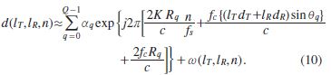
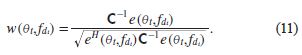
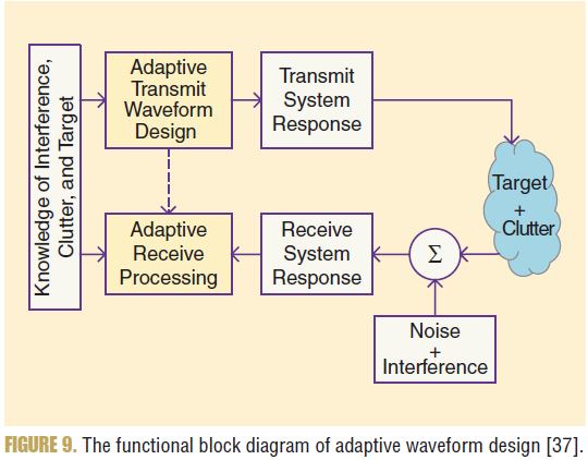
[37] L. K. Patton and B. D. Rigling, “Modulus constraints in adaptive radar waveform design,” in Proc. IEEE Radar Conf., 2008, pp. 1–6.

[38] M. R. Bell, “Information theory and radar waveform design,” IEEE Trans. Inform. Theory, vol. 39, no. 5, pp. 1578–1597, Sept. 1993.

[39] Y. Yang and R. S. Blum, “MIMO radar waveform design based on mutual information and minimum mean-square error estimation,” IEEE Trans. Aerosp. Electron. Syst., vol. 43, no. 1, pp. 330–343, Jan. 2007.

[40] A. Leshem and A. Nehorai, “Information theoretic radar waveform design for multiple targets,” in Proc. Int. Waveform Diversity and Design Conf., Pisa, Italy, 2007, pp. 362–366.

[41] D. Kok and J. S. Fu, “Signal processing for automotive radar,” in Proc. IEEE Int. Radar Conf., Arlington, VA, 2005, pp. 842–846.

[42] H. Rohling, “Radar CFAR thresholding in clutter and multiple target situations,” IEEE Trans. Aerosp. Electron. Syst., vol. 19, no. 4, pp. 608–621, July 1983.

[43] J. Ward, “Space-time adaptive processing for airborne radar,” in Proc. Int. Conf. Acoustics, Speech and Signal Processing, London, U.K., 1995, vol. 5, pp. 2809–2812.

[44] M. C. Wicks, M. Rangaswamy, R. Adve, and T. B. Hale, “Space-time adaptive processing: A knowledge-based perspective for airborne radar,” IEEE Signal Process. Mag., vol. 23, no. 1, pp. 51–65, Jan. 2006.

[45] V. F. Mecca, D. Ramakrishnan, and J. L. Krolik, “MIMO radar space-time adaptive processing for multipath clutter mitigation,” in Proc. IEEE Workshop Sensor Array and Multichannel Processing, Waltham, MA, 2006, pp. 249–253.

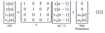
[46] A. Macaveiu, A. Campeanu, and I. Nafornita, “Kalman-based tracker for multiple radar targets,” in Proc. Int. Conf. Communication, Bucharest, Romania, 2014, pp. 1–4.

[47] S. M. Kay, Fundamentals of Statistical Signal Processing: Estimation Theory. Upper Saddle River, NJ: Prentice-Hall, 1993.

[48] M. Z. Ikram and M. Ali, “3-D object tracking in millimeter-wave radar for advanced driver assistance systems,” in Proc. IEEE Global Conf. Signal and Information Processing, Austin, TX, 2013, pp. 723–726.

[49] A. Macaveiu and A. Câmpeanu, “Automotive radar target tracking by Kalman filtering,” in Proc. Int. Conf. Telecommunication Modern Satellite, Cable and Broadcasting Services, Nis, Serbia, 2013, vol. 2, pp. 553–556.

[50] D. Oprisan and H. Rohling, “Tracking systems for automotive radar networks,” in Proc. RADAR, Edinburgh, U.K., 2002, pp. 339–343.

[51] N. Floudas, A. Polychronopoulos, and A. Amditis, “A survey of filtering techniques for vehicle tracking by radar-equipped automotive platforms,” in Proc. IEEE Int. Conf. Information Fusion, Philadelphia, PA, 2005, vol. 2, pp. 1436–1443.

[52] V. C. Chen, F. Li, S. S. Ho and H. Wechsler, “Micro-Doppler effect in radar: Phenomenon, model, and simulation study,” IEEE Trans. Aerosp. Electron. Syst., vol. 42, no. 1, pp. 2–21, Jan. 2006.

[53] H. Rohling, S. Heuel, and H. Ritter, “Pedestrian detection procedure integrated into an 24 GHz automotive radar,” in Proc. IEEE Radar Conf., Washington, DC, 2010, pp. 1229–1232.

[54] N. Yamada, Y. Tanaka, and K. Nishikawa, “Radar cross section for pedestrian in 76 GHz band,” in Proc. IEEE European Microwave Conf., Paris, France, 2005, vol. 2, pp. 4–8.

[55] D. M. Gavrila, “Sensor-based pedestrian protection,” IEEE Intell. Syst., vol. 16, no. 6, pp. 77–81, 2001.

[56] M. Bertozzi, A. Broggi, A. Fascioli, A. Tibaldi, R. Chapuis, and F. Chausse, “Pedestrian localization and tracking system with Kalman filtering,” in Proc. IEEE Intelligent Vehicles Symp., Detroit, MI, 2004, pp. 584–589.

[57] L. Ding, M. Ali, S. Patole, and A. Dabak, “Vibration parameter estimation using FMCW radar,” in Proc. IEEE Int. Conf. Acoustics, Speech and Signal Processing, Beijing, China, 2016, pp. 2224–2228.

[58] T. Thayaparan, S. Abrol, and E. Riseborough, “Micro-Doppler radar signatures for intelligent target recognition,” DTIC Document, Tech. Rep., 2004.

[59] Y. Li, L. Du, and H. Liu, “Moving vehicle classification based on micro-Doppler signature,” in Proc. IEEE Int. Conf. Signal Processing, Communications and Computing, Xian, China, 2011, pp. 1–4.

[60] Advanced design system. [Online]. Available: http://www.keysight.com/en/ pc-1297113/advanced-design-system-ads

[61] Feko Homepage [Online]. Available: https://www.feko.info/

[62] D. Andersh, J. Moore, S. Kosanovich, D. Kapp, R. Bhalla, R. Kipp, T. Courtney, A. Nolan, F. German, J. Cook, and J. Hughes, “Xpatch 4: the next generation in high frequency electromagnetic modeling and simulation software,” in Proc. IEEE Radar Conf., Alexandria, VA, 2000, pp. 844–849.

[63] D. Göhring, M. Wang, M. Schnürmacher, and T. Ganjineh, “Radar/lidar sensor fusion for car-following on highways,” in Proc. Int. Conf. Automation, Robotics and Applications, Wellington, New Zealand, 2011, pp. 407–412.

[64] R. H. Rasshofer and K. Gresser, “Automotive radar and lidar systems for next generation driver assistance functions,” Adv. Radio Sci., vol. 3, pp. 205–209, May 2005.

[65] M. Mahlisch, R. Hering, W. Ritter, and K. Dietmayer, “Heterogeneous fusion of video, LIDAR and ESP data for automotive ACC vehicle tracking,” in Proc. IEEE Int. Conf. Multisensor Fusion and Integration for Intelligent Systems, Heidelberg, Germany, 2006, pp. 139–144.

[66] B. Steux, C. Laurgeau, L. Salesse, and D. Wautier, “Fade: A vehicle detection and tracking system featuring monocular color vision and radar data fusion,” in Proc. IEEE Intelligent Vehicle Symp., Versailles, France, 2002, vol. 2, pp. 632–639.

[67] P. Viola and M. Jones, “Robust real-time object detection,” Int. J. Comput. Vis., vol. 4, Feb. 2001.

[68] G. M. Brooker, “Mutual interference of millimeter-wave radar systems,” IEEE Trans. Electromagnet. Compat., vol. 49, no. 1, pp. 170–181, Feb. 2007.

[69] P. Papadimitratos, A. D. La Fortelle, K. Evenssen, R. Brignolo, and S. Cosenza, “Vehicular communication systems: Enabling technologies, applications, and future outlook on intelligent transportation,” IEEE Commun. Mag., vol. 47, no. 11, pp. 84–95, Nov. 2009.

[70] F. Ye, M. Adams, and S. Roy, “V2V wireless communication protocol for rear-end collision avoidance on highways,” in Proc. IEEE Int. Conf. Communication Workshop, Beijing, China, 2008, pp. 375–379.