
In an earlier version of our paper [1], a general introduction to Residue Number System based arithmetic [2] [3] [4] [5] [6] has been presented. In this continuation article, we give a tutorial on the design of a RNS based processor for specific application in Digital filtering. The most popular application of RNS is in the design of FIR (Finite Impulse Response) filters.
In the case of FIR filters (see Figure 1), we need to perform several multiplications of present sample and previous input samples x(n) with fixed coefficients h(n) defining the impulse response of the filter and accumulate the results of these multiplications to obtain y(n):
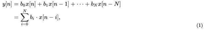
Note that N is the number of taps of the FIR filter.
We need to convert input samples to RNS form whenever sample is available and these residues need to be stored in a RAM. The binary to RNS conversion takes a time of ΔFC. (FC stands for Forward Converter). The coefficients which are in binary form also need to be converted into residue form and stored in ROM. This is done only once, after the FIR filter is designed using some DSP filter design programs like in MATLAB tool box. We need to read the RAM and ROM contents and multiply the residues in separate i Residue processors. This needs modulo multipliers to compute (a×b) modulo mi where mi is i-th modulus. After each multiplication, we need to accumulate the residues in modulo mi adders. This MAC (Multiply and Accumulate) operation needs to be carried out N times for a N-tap FIR filter. After this computation we need to convert the resulting residues corresponding to y(n) into conventional binary form using a RNS to Binary converter. Since in each sample clock period, N modulo multiplications and modulo accumulations (additions with previous stored sum) need to be carried out, we need a computation time of N× ΔMACR where subscript R stands for residue Multiply and Accumulate (MAC) operation. The total computation time is thus ΔFC+ N×ΔMACR+ ΔRC where ΔFC is the time or forward conversion and ΔRC is the time for reverse conversion. This may be compared with computation using conventional DSP which is N×ΔMAC. Typically modern DSPs have 16 bit × 16 bit multipliers and an accumulator of width 40 bits. This means that 256 MAC operations can be performed very accurately and after the computation the result can be truncated or rounded off and taken as 16 bit word. To be competitive, RNS processors also shall have similar dynamic range for the accumulated result of 40 bits whereas the operands to be multiplied are 16 bits. We start with this design problem.
For having a 40 bit dynamic range, we can choose RNS of several moduli. If we consider three moduli set {2n-1, 2n, 2n+1}, we have dynamic range slightly more than 40 bits by choosing n = 14. In other words we have three processors working with bit lengths 14, 14 and 15 bits for the three moduli {214-1, 214, 214+1}. You can see the decrease in word length from 40 bits to 14 bits for each accumulator. If we consider this to be large, we can choose a four moduli set among several options available for example
{2n-1, 2n, 2n+1, 2n+1-1} with n = 10 i.e. the moduli are {1023,1024,1025, 2047} which reduces the word length of each residue processor from 14 bits to 10 bits. Alternatively, we can choose a five moduli set
{2n-1, 2n, 2n+1, 2n+1-1, 2n-1-1} with n = 8 i.e. the moduli are {255,256,257,511,127}. Evidently, the word length is 8 to 9 bits. Note that the moduli need to be mutually prime. We need thus modulo adders of 8, 8, 9, 9 and 7 bits respectively for the five moduli set. We also need modulo multipliers for these word lengths. We will now describe each of the building blocks.
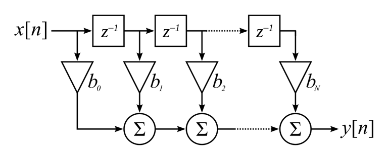
Figure 1: A N-tap FIR filter
We need to find (A+B) mod mi where mi is the modulus and bi bits are used to represent mi i.e. bi = ⌈log2mi⌉. Normally, we need to find C1 = (A+B) first and then subtract mi from C1 to get C2 = (A+B-mi). Then the answer Z is C1 or C2 depending on the sign of C2. Thus the computation time is that two bi-bit additions. The hardware requirement is two bi-bit adders and one Multiplexer (see Figure 2 (a)). Note, however, you can simplify hardware in case of special mi which we have considered above. In case of modulus 2n, we need one adder but we can ignore the carry. As an example for modulus 16, A = 10, B = 13 gives C1 = 23 = 101112= 0111 ignoring carry since (23) mod 16 = 7. Note that (subscript 2 indicates binary number). In case of modulus (2n-1) also, the second adder can be removed and instead we feedback the carry of adder 1 to carry input once again and add. Note that we have used the fact that 2n mod (2n-1) = 1. This adder shown in Figure 2(b) is called end-around-carry adder. The addition time is same as before since only after carry of first addition is available, another addition can be performed. Subtraction is similar to addition with the difference that we compute C3 = A-B and C4 = A-B+mi and select C3 or C4 based on the fact whether C3 is negative. (We need to add two’s complement of B to A i.e. invert the bits of B and add 1). In the case of modulus (2n+1), we can use the architecture of Figure 2(a) and we need a (n+1) bit adder 1 and (n+2) -bit adder 2.
We can use conventional multiplier (see Figure 3(a) first to find (A×B) and then find residue mod mi. Multiplication mod 2n is simple since we need to take only n LSBs of the product. As an illustration, consider finding (5×13) mod 16 = 1 since the product 65 = (0100 0001)2 and we ignore the four MSBs. Multiplication mod (2n-1) can be done in several ways. One method finds (A.B) first and then we add MSBs with LSB using an end-around-carry (EAC) adder. For the same example above, we have
5×13 mod 15 = 65 mod 15 = (0100 0001)2 mod 15 = (1+4) mod 15 = 5.
We can use the EAC adder of Figure 2(b) on the product (A.B). The multiplication time is sum of normal multiplication time followed by modulo 15 reduction time.
In the case of modulus (2n+1), we need to subtract MSBs of the product (A.B) from LSBs of the product and if the result is negative we need to add (2n+1). As an illustration, consider (5×13) mod 17 = (0100 0001) mod 17 = (1-4) mod 17 = 14.
Note however, that there are other elegant methods for modulo multiplication where we make use of the properties of the moduli (2n-1) and (2n+1) [5]. We demonstrate this method in the case of mod (2n-1) multiplication. We use the well-known shift and add method of multiplication with a difference. The partial products in conventional shift and add extend beyond n bits for a n×n multiplication. In case of mod (2n-1) multiplication, we write the bits beyond the MSB positions in LSB positions. This is because of the fact that (a×2n) mod (2n-1) = a. Thus we get a square array of words which we add using a chain of Carry Save Adders (CSA) with end around carry followed by a Carry Propagate Adder (CPA). We are reducing the carry bit C of weight 2n mod (2n-1) as LSB of value C. The method can be understood by looking at the Figure 3(b) for an example (11×13) mod 15. Evidently, there will be n number of n-bit words for adding which we need (n-2) levels and finally, the carry and sum vectors are added using an adder of type Figure 2(b). (see Figure 3(c)). The multiplication time is thus (n-2) DFA for carry save adders and 2n DFA for the final Carry propagate adder (CPA) where DFA is a full-adder delay.
In the case of mod (2n+1) multiplication, which is involved slightly, we use another property (a×2n) mod (2n-1) = –a. Thus the MSBs of the partial products need to be subtracted from n LSBs. We realize this by adding one’s complementing (inverting all the bits) of the MSB word and adding a correction term. This can be understood as follows. If we want to subtract the 3 bit MSB word of value 5 = (101)2 , we write it as one’s complement i.e. 010 which means that we have added 7 since -5 is implemented as 7-5. We need hence to subtract 5 at the end. This operation applies to all the MSB words. The total quantity we have added is 13. Hence if we add 4, we would have added 17 where mod 17 is zero. We again present an example (11×13) mod 17 in Figure 3(d). This needs one final correction term to be added thus needing one more level in the carry save adder chain and final mod (2n+1) reduction.
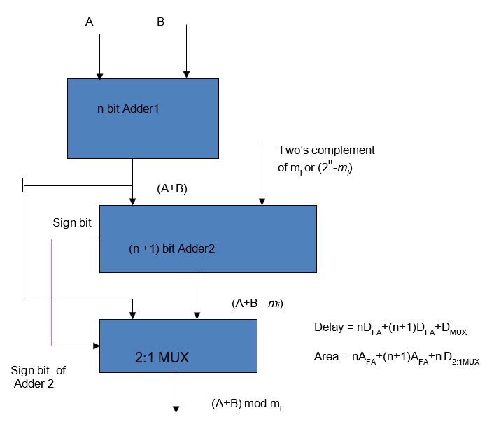
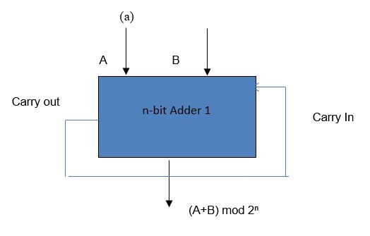
Figure 2 (a) A modulo mi adder (b) modulo (2n-1) adder
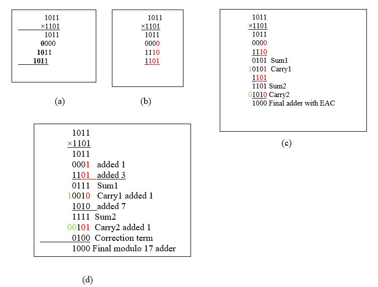
Figure 3 (a) Normal multiplier (b) rewritten to perform mod 15 multiplication (c) Actual realization using Carry save adders and final EAC adder (d) mod 17 multiplier
With these blocks now we are ready regarding FIR filter computation provided input residues are given. The input residues corresponding to given input binary words can be easily obtained for the various moduli as follows: The residue mod 2n for a 3n-bit number is n least significant bits itself. The residue mod (2n-1) can be obtained by adding the three n –bit words in the given 3n-bit number. Considering the given number as X = a.22n+b.2n+c, we have residue mod (2n-1) as r2 = (a+b+c) mod (2n-1).
As explained before, we can add the three words in a CSA followed by a CPA with EAC. In the case of modulus (2n+1), we find (a-b+c) mod (2n+1). We add a and c with two’s complement of b and the result if negative, we add 2n+1. If the result is positive, we subtract 2n+1. As an illustration, suppose we consider moduli 16, 15 and 17 and given 12 bit word is 1001,0100,11002, we compute r1, r2 and r3 as r1 = 12, r2 = (9+4+12) mod 15 = 10 and r3 = (9-4+12) mod 17 = 0. The reader may verify this to be true since input given decimal number is 2380.
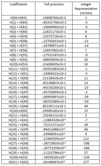
We will next describe a 64 tap FIR filter implementation using the example from Jenkins and Leon [6] whose coefficients are given in Table. The coefficients are scaled to get the integer part. The filter takes 64 input samples and weighs them using the tap weights given in Table I and finds the sum. We need to estimate the worst case maximum of the sum of product of coefficients and all samples to be of maximum value say 8 bits with one sign bit as 2784×128 = 356,352 corresponding to 18.44 bits. This dynamic range (DR) can be met by choosing for example four moduli as 15, 16, 17 and 31. The DR achievable is 2,127,840 (> 20 bits). Thus, we need four Binary to RNS converters, 4 RNS accumulators (mod mi adders), 4 RNS multipliers and finally one RNS to Binary converter. The computation time is ΔFC+ 64ΔMAC+ ΔRC. The one of the reverse converters described in literature can be used. Alternatively, a three moduli RNS can be used with moduli 127,128 and 129 yielding DR of 21 bits. One needs to assess the total area requirements and largest MAC time and decide on the choice of moduli set. Note that since we have considered worst case dynamic range, no need for scaling arises.
Table I. Coefficients of FIR filter
Using small building blocks such as Modulo adders, subtractors, multipliers, efficient processors for custom VLSI DSP applications can be designed. It has been shown in literature that the use of RNS can lead to low power designs as well. Of late, several applications in cryptography have benefited from the use of RNS to crunch extremely large numbers. We have considered the design of FIR filters but the techniques described can be extended to IIR filters as well.
[1] P. V. Ananda Mohan, Residue Number systems: A Primer, Advanced Computing and Communications, Vol.1, pp 46-52, June 2017
[2] N. S. Szabo and R. I. Tanaka, Residue Arithmetic and Its Applications to Computer Technology, New-York: Mc-Graw Hill, 1967.
[3] M. A. Soderstrand, G. A. Jullien, W. K. Jenkins and F. Taylor, (Eds), Residue Number System Arithmetic: Modern Applications in Digital Signal Processing, IEEE Press, 1986.
[4] A. Omondi and A. B. Premkumar, Residue Number System Theory and Implementation, vol. 2, Imperial College Press, 2007.
[5] P. V. Ananda Mohan, Residue Number Systems: Theory and Applications, Switzerland: Birkhauser, 2016.
[6] W. K. Jenkins and B. J. Leon, “The use of residue number systems in the design of finite impulse response digital filters”, IEEE Transactions on Circuits and Systems, Vol. CAS-24, pp 191-201, 1977.