In Part I we laid the foundation on which quantum algorithms are built. In this part we harness such exotic aspects as superposition, entanglement and collapse of quantum states of that foundation to show how powerful quantum algorithms can be constructed for efficient computation. Appendixes A and B are provided to jog the memory of those who are recently out of touch with linear algebra and Fourier series.
NOTE: Readers desirous of getting some hands-on experience with a few of the algorithms presented in Part II can visit https://acc.digital/Quantum_Algorithms. This material is provided by Vikram Menon using the IBM Q Experience for Researchers. (see https://quantumexperience.ng.bluemix.net/qx/experience” ).
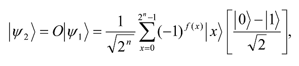
Developers of quantum algorithms must always bear in mind an intriguing aspect of Nature. It keeps track of all the continuous parameters describing the state of a quantum system, like a and b that describe, say, the state |Ψâ© = a|0â© + b|1â© of a qubit, but keeps most of that information hidden from observers. Nature hides information or more likely we are not smart enough to discover it.
In quantum computation, the state of the quantum computer is described by a state vector |Ψâ©, which in its general form is a complex linear superposition of all binary states of the qubits. The temporal evolution of |Ψâ© is described by a unitary operator U on this vector space.
The unique ability of qubits to stay in superposed and entangled states and the ability of unitary operators to act in parallel on all the superposed states of one or more qubits, permits some unusual computational tricks. For example, it is possible to calculate the value of a function f(x) for multiple values of x in parallel without parallel replication of computing hardware. Indeed, quantum parallelism comes for free. Further, the Hadamard gate generates genuine random numbers. The essence of designing quantum algorithms lies in the clever use of quantum superposition of states, entanglement of quantum states, wave interference, and collapse of quantum states.
The design of quantum algorithms lies in the clever choice of computational and measurement bases, initial states, sequence of unitary gates and measurement points. Certain things, e.g., determination of global information about a function, is more efficiently done than on classical computers.
Random number generation
When we think of random numbers we think of tossing a fair coin. Quantum particles can be made the fairest coins of all. Random numbers can be generated perfectly by preparing a qubit in state |0â© or |1â© and applying the Hadamard gate to change its state to (|0â© + |1â©)/√2 or (|0â© -|1â©)/√2, respectively, and then measuring the state. The result will be either |0â© or |1â© with equal probability.
n-qubit Hadamard gate
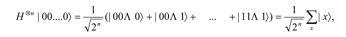
When the Hadamard gate is applied to n qubits individually, we get
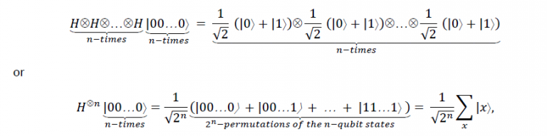
where the sum is over all possible 2n mutually orthogonal states of n qubits or values of x. Thus, the Hadamard transform produces an equal superposition of all 2n possible computational basis states, i.e., x can be viewed as the binary representation of the numbers from 0 to 2n -1. The n-qubit Hadamard gate is sometimes known as the Walsh-Hadamard gate.
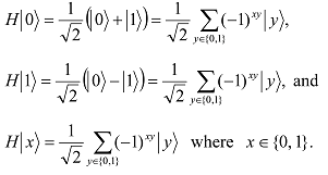
Consider a single qubit in state |xâ© where x ∈ {0, 1}. Then
For an n-qubit system |xâ© = |x1â©…|xnâ© = |x1 … xnâ©, we have
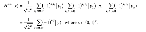
x·y is the bitwise inner product of x and y modulo 2 and |yâ© = |y1â© …|ynâ© = |y1 … ynâ©. The reader should instinctively spot the above formula (last line) as it will appear frequently in later Sections.
Take 3 qubits, each prepared in state |0â©. The first qubit is the placeholder for x, the second for y, and the third for the result of x∧y. To create the 4 possible inputs of x and y, {|00â©, |01â©, |10â©, |11â©}, apply the Hadamard gate to the first two qubits to get
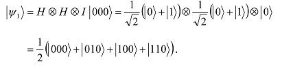
An application of the Toffoli gate, T, then produces
![]()
Notice that the 3-qubit system is put into equal superposition of the four possible results of x∧y. The result of ANDing the first two qubits appears in the third qubit.
By applying the Cnot gate to the first two qubits of T|Ψ1â© above we get
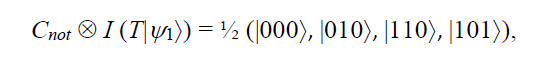
where the second qubit is the sum and the third qubit is the carry bit. Note that the carry bit in the adder is the result of an AND operation. The carry and AND are really the same thing. The sum bit comes from an XOR gate (that is, the Cnot operation).
Three applications of the Cnot gate will swap |a, bâ© to |b, aâ©:
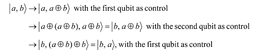
where ⊕ denotes modulo 2 addition2
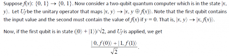
Pay very careful attention to this landmark algorithm in quantum computing. Consider the Boolean functions f that map {0, 1} to {0, 1}. There are exactly four such functions, as follows:
(1) two “constant” functions: f(0) = f(1) = 0 and f(0) = f(1) = 1;
(2) two “balanced” functions: f(0) = 0, f(1) = 1 and f(0) = 1, f(1) = 0.
The task is to identify the set to which f(0) and f(1) belong to in only one measurement. Note, that we do not seek the values of f(0) and f(1) but only a global property of f.
The solution provided here is reported in Cleve, et al3., which improves upon the original paper by Deutsch (1985)4. Deutsch’s solution had three possible outcomes: “balanced”, “constant”, and “inconclusive” with 50% probability that it would produce an “inconclusive” result. The solution described here always correctly identifies “constant” and “balanced” functions. The improvement took more than a decade to be discovered.
Let the initial state of the 2-qubit system be |Ψâ© = |01â© . When the Hadamard gate acts on it, we get
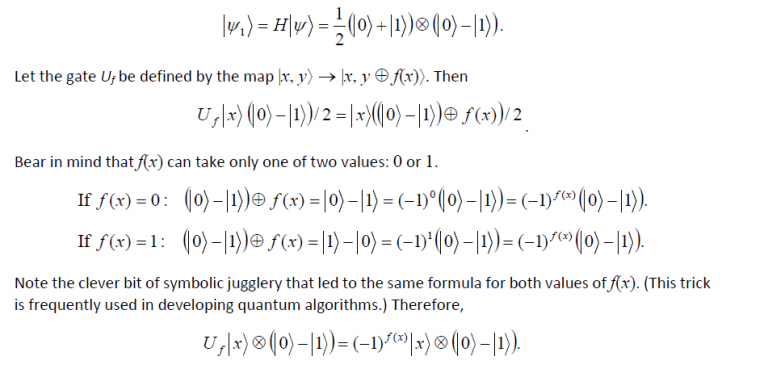
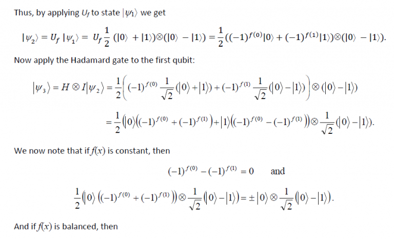
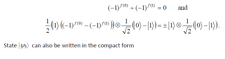
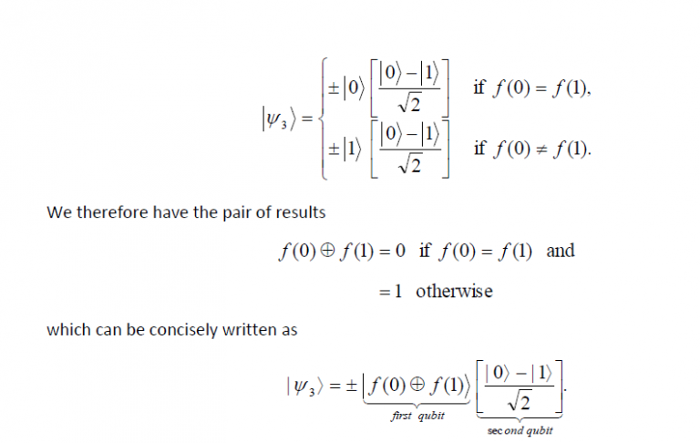
What has been cleverly accomplished is that by measuring the first qubit we may determine f(0) ⊕ f(1) which will tell us if f(0) = f(1) or not. In essence, just one evaluation of f(x) has allowed us to find a global property of f(x), namely, f(0)⊕ f(1). On the other hand, a classical computer would have required at least two evaluations. The Deutsch algorithm provided the first example that a quantum computer could do something that a classical computer cannot. It was simply brilliant in conception.
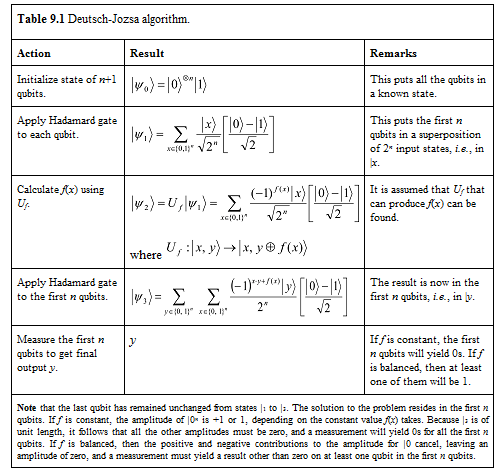
The Deutsch-Jozsa algorithm5 solves a generalized Deutsch problem. Given a black box Uf whose action is to perform |x, yâ© |x, y ⊕ f(x)â© for x ∈ {0, 1} n ≡{0,…,2n -1} and f(x)∈ {0, 1}, and that it is known beforehand that f is one of two kinds: either f(x) is constant for all values of x, or else f(x) is balanced, i.e., equal to 1 for exactly half of all possible x, and 0 for the other half. The significance of this problem is that a classical solution, in the worst-case, would require 2n-1 +1 evaluations of f before determining the answer with certainty since one may receive 2n/2 0s before finally getting a 1. Remarkably, the Deutsch-Jozsa algorithm requires only one evaluation of f. The reader is encouraged to see Table 9.1 where the algorithm is provided in summary form.
The Deutsch–Jozsa algorithm later inspired two revolutionary quantum algorithms, namely Shor’s factoring algorithm and Grover’s search algorithm, described in Section 10.
This is remarkable. The first term contains information about f(0) along with its input x = 0, and the second term contains information about f(1) along with its input x = 1. That is, the second qubit is in an equal superposition of f(0) and f(1), and the two values were calculated in parallel. This power of quantum algorithms comes from quantum parallelism and entanglement. So, most quantum algorithms begin by computing a function f(x) on a superposition of all values of x as follows:
Start with an n-qubit state |00…â© and apply H to all the qubits to get
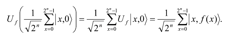
which is the superposition of all integers 0≤ x < 2n. Next, add a k-qubit register in state |00..0â©, large enough to hold the longest value of f(x). Then by linearity
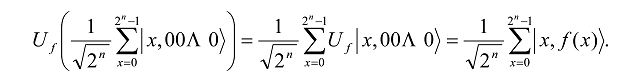
Thus f(x) is computed in parallel for all values of x∈ {0,…, 2n -1}, provided one knows how to construct the appropriate Uf that will map a pair of qubit strings |x, 0â© into the pair |x, f(x)â©. The output comes from the constructive interference of parallel computations.
The trick in constructing Uf is to break down the computation, corresponding to the function f(x), into a set of 1-qubit and 2-qubit unitary operations such that the state |xâ©, 0 is mapped to the state |x, f(x)â© for any input x. Note that the number of qubits required for the second register must be at least sufficient to store the longest result f(x) for any of these computations. In general, in designing quantum algorithms, one assumes that for reasonable functions, a suitable Uf can be built.
2 0 ⊕ 0 = 0, 0 ⊕ 1 = 1, 1 ⊕ 0 = 1, 1 ⊕ 1 = 1. See Sec. A.5.7 in Appendix A for a quick recall of modular arithmetic.
3Cleve, et al (1998).
4 Deutsch (1985).
5 Deutsch & Jozsa (1992).
The problem and its solution were proposed by Avshalom Elitzur and Lev Vaidman in 19936. Consider a bomb with an ultra-sensitive detonator on its nose that even a photon impinging on the detonator’s slightly wobbly mirror can set it off (see Fig. 9.1). The bomb’s production line is not perfect—in some cases the detonator is jammed, and the bomb fails to explode and is classed a dud. The problem is to determine if a bomb’s plunger is stuck or not without exploding the bomb. Classical physics cannot determine without exploding the bomb. The solution is an interesting application of the Mach-Zehnder interferometer. The photon source emits a single photon. Now two possible paths for the photon exist.
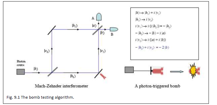
If the photon takes the |h1â© path (50% probability), the bomb’s mirror will either absorb the photon and wobble and the bomb will explode, or it will simply send the photon along the |v2â© path because the plunger is stuck and the photon will be detected by the detector B. In this case 50% of good bombs will explode.
The more interesting case is when the photon takes the |v1â© path (50% probability). The photon then does not impinge on the bomb’s mirror and so even a good bomb cannot explode. But the photon’s superposed state will still sense if the |h1â© path has a wobbly mirror or not! If it senses a jammed mirror, the photon will end up at detector B. If it senses a wobbly mirror, it can end up at either detector A or at B. Note that if A detects a photon then the bomb is not a dud. Thus, in half of the cases where an active bomb does not explode will the detector A register a photon. At the end of the tests, we would have found only a quarter of the originally active bombs which are guaranteed to be actually still active. We can continue to repeat the tests on the remaining doubtful bombs till no doubtful bomb is left. Ultimately, we will obtain just one third (since 1/4 + 1/16 + 1/64 +… = 1/3) of the active bombs that we started with, but they are now guaranteed to be active.
Quantum advantage: Classically there would be no way of saving even a single good bomb, but quantum mechanically one can save one third of them. With some refinements, the two-thirds wastefulness can be reduced effectively to one-half (Elitzur and Vaidman, 1993)7. In 1995, Kwiat, Weinfurter, Herzog, and Zeilinger reported an experiment verifying the Elitzur-Vaidman result, thus proving that interaction-free measurements are indeed possible8. The same year, Kwiat, Weinfurter, Zeilinger, Herzog, and M. Kasevich devised a method, using a sequence of polarizing devices, which efficiently increased the yield rate to a level arbitrarily close to one9.
6 Elitzur & Vaidman (1993). See also: Penrose (1994), pp. 239-240 and 268-270;
and Baeyer (2001), p. 16.
7 Elitzur & Vaidman (1993).
8 Kwiat, et al (1995a). See also: Kwiat, et al (1995b).
9 Kwiat, et al (1995c). See also: DeWeerd (2002).
The exchange of secret messages in a completely secure manner requires a perfect cypher such as the Vernam cypher10 or one-time pad invented in 1917. Unfortunately, it requires a key equal in size to the plain text message and Shannon’s information theory11 says it cannot be reduced without compromising security. Thus, distributing the key itself, especially for voluminous data, e.g., bank transactions, is a problem since the key must be sent over a secure channel. In practice, less secure methods, such as the RSA public key cryptosystem12 are often used.
In 1984, Charles H. Bennett and Gilles Brassard described the first completely secure quantum key distribution algorithm, now known as the BB84 protocol13. It relies on the Hadamard operator to create random numbers, and the fact that a quantum system collapses when measured. Thus, an eavesdropper intercepting a message will invariably make its presence known as a disturbance in the key distribution channel. Quantum entanglement is not used in the BB84 protocol, yet it is so secure that encrypted messages can be sent publicly.
In the protocol, suppose Alice and Bob want to communicate privately, and Eve wants to eavesdrop. Their available means of communication are an ordinary bidirectional open channel (e.g., a telephone) and a unidirectional quantum channel. Both channels can be intercepted. The quantum channel allows Alice to send individual photons to Bob who can measure their quantum state. Eve may measure the state of these photons and resend them to Bob. To establish the key Alice begins by sending Bob a sequence of encoded photons. For encoding, Alice randomly uses one of the following two bases:![]()
where the arrows indicate the polarized state of the photon used to encode the binary digits 0 and 1. Bob measures the state of the photons he gets by randomly picking either basis. After the qubits have been transmitted and measured, Alice and Bob communicate, over the open channel, the basis they used for coding and decoding of each bit. (This amounts to sending a string of symbols, which are meaningless without the measurements themselves.) On average, 50% of the time their bases will match. Alice and Bob use those photons as the key for which their bases agree and discard the other photons. So far nothing has been gained by using qubits.
Can Eve steal the key? Suppose Eve measures the state of the photons sent by Alice and resends new photons with the measured state to Bob. However, being unaware of the basis sequence used by Alice, Eve will get her measurement basis wrong, on average, 50% of the time. Thus, when Bob measures a resent photon with the correct basis (Alice’s basis) there will be a 25% probability that he will measure the wrong value. This is because Eve, by measuring the photons en route, would have collapsed them to her measured value. Thus, Eve is bound to introduce a high rate of error that Alice and Bob can detect by communicating a sufficient number of parity bits of their keys over the open channel. So, not only will Eve’s version of the key will be, on average, 25% incorrect, but that someone is snooping will be apparent to Alice and Bob. If so detected, Alice and Bob simply discard the key and send a new one. Only when both are certain that their key is uncompromised will they use it for encryption. Their encrypted messages can now be broadcast if you please.
Later, Bennett14 found a fiberoptic interferometric version of the quantum key distribution method, and then Bennett and Wiesner15 developed a method that uses macroscopic signals instead of single photons thereby solving the problem of stray light and lowering the cost of the device by using signals which are more efficient and less noisy than photon counting detectors at the wavelengths where optical fibers are most transparent. Both methods were patented.
We now come to more complex algorithms, mainly Peter Shor’s highly efficient algorithm for finding the prime factors of an integer, and Lov Grover’s search algorithm which efficiently conducts a search through unstructured search spaces. Both algorithms were breakthroughs, in terms of computational efficiency in comparison to the best known classical algorithms for either problem, and in terms of conceptual ideas. It is all about managing the relative phase factors using unitary operators.
Recall that the basis independent global phase factors do not affect measurement, hence they can be ignored. Only states, which differ by relative phases in some basis, give rise to physically observable differences in measurement. Therefore, the key to algorithm design is manipulating relative phase as we just saw in Sec. 9.8 using the Mach-Zehnder interferometer. Further, algorithms described in this section depend heavily on quantum entanglement. Note further that it is assumed that given a function f(x), it is possible to break down its computation to the application of a set of one-qubit and two-qubit unitary operations. Typically, the sequence of operations is designed to map the state |x, 0â© to the state |x, f(x)â© for any input x. The number of qubits required to represent x and f(x) are appropriately chosen before starting the computations.
Fourier transforms map from the time domain to the frequency domain. In other words, they map functions of period r to functions that have non-zero values only at multiples of the frequency 2π/r. The discrete Fourier transform (DFT) operates on N equispaced samples in the interval [0, 2π] for some N and outputs a function whose domain is the integers between 0 and N-1. The DFT of a sampled function of period r is a function concentrated near multiples of N/r. If the period r divides N evenly, the result is a function that has non-zero values only at multiples of N/r. Otherwise, the result will approximate this behavior, and there will be non-zero terms at integers close to multiples of N/r. In the special case when N is a power of 2, the DFT results in a version known as the Fast Fourier transform (FFT).
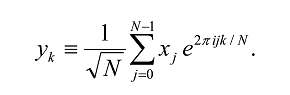
The discrete Fourier transform takes as input a vector of complex numbers, x0 , x1, …, xN-1 where N is a fixed positive integer, and outputs another vector of complex numbers y0 , y1, …, yN-1 defined by
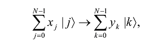
The quantum Fourier transform (QFT) is exactly the same transform. When written in the Dirac notation on an orthonormal basis |0â© , …, |N-1â© , it is defined to be a linear operator with the following action on the basis states16,
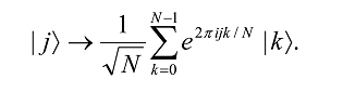
Equivalently, the action on an arbitrary state may be written as
where the amplitudes yk are the discrete Fourier transform of the amplitudes xj, and k and j both range over the binary representations for the integers between 0 and N-1. We see that it corresponds to a vector notation for the Fourier transform (first equation of this subsection) for the case N = 2n. If the state is measured after the Fourier transform is performed, the probability that the result will be |kâ© is |yk|2. Note that the QFT does not output a function the way the Uf transformation does, i.e, no output appears in an extra register. It can be shown that QFT is unitary.
The best classical algorithms for computing the discrete Fourier transform of 2n elements such as the Fast Fourier Transform (FFT), take roughly N log(N) = n2n steps to Fourier transform N = 2n numbers. On a quantum computer, it takes about log2(N) = n2 steps, an exponential reduction! Of course, we need to deal with the fact that the results of such parallel calculations are not readily accessible.
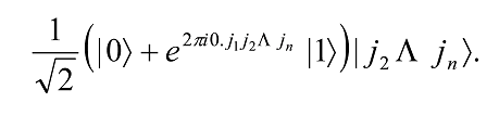
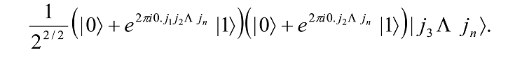
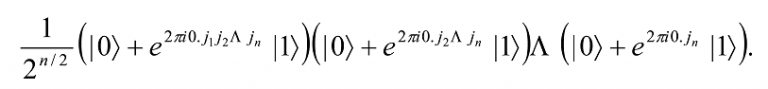
If we take N = 2n, where n is some integer17, and |0â©, …, |2n – 1â© as the computational basis for an n-qubit quantum computer, it is convenient to write the state |jâ© using the binary representation j = j1 j2 … jn as a shorthand for j = j12n-1 + j22n-2 + … + jn20 and likewise the notation 0.j1 j2 … jm as a shorthand for the binary fraction j1/2 + j2/22 + … + jm/2m. Then
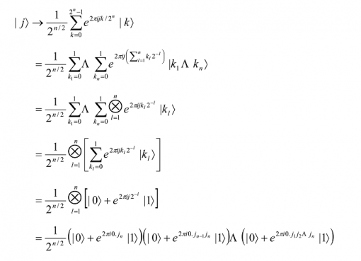
Thus, we have
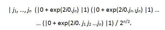
The above product representation shows the state is unentangled and may even be viewed as an alternative definition of the quantum Fourier transform. It is particularly useful when visualizing the unitary transformations needed to form them. For example, it is obvious that unitary gates of the form
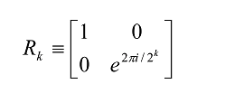
are expected to play a role.
Let us see what sequence of unitary gates allows the QFT to be calculated. Take the state | j1 … jnâ© as input. An application of the Hadamard gate to the first qubit produces the state
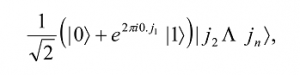
since e2πi0j1= -1 when j1=1, and +1 otherwise. Now an application of the controlled-R2 gate (this is a conditional rotation) produces the state
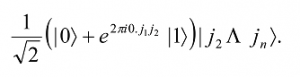
By continuing with the controlled-R3, R4 through Rn gates, we successively add an extra bit to the phase of the coefficient of the first |1â©. In the end the resulting state is
Next, we perform a similar procedure on the second qubit, namely, the application of a Hadamard gate followed by controlled-R2 through Rn-1 gates, to obtain
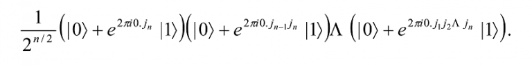
By continuing in this fashion for each successive qubit, we get the final state
Finally, the swap operation (see Section 9.4) is used to reverse the order of the qubits to provide the final result
On a quantum computer the Fourier transform can be done using O(n2) gates18. This spectacular reduction in computational steps is not feasible on a classical computer even for rather small values of n. The importance of QFT is that many quantum algorithms seem to follow the generic sequence: a Fourier transform, followed by a f-controlled-U, followed by another Fourier transform, or has this sequence as an important component.
10 Developed by Gilbert Vernam of AT&T. This is the only known totally secure cipher.
11 See, e.g., Goldreich (2004). See also: Black, Kuhn & Williams (2002), Sec. 5.
12 Rivest, Shamir & Adleman (1978). Rivest, Shamir, and Adleman received the Turing award for 2002 for their contributions to public key cryptography. http://www.acm.org/announcements/turing_2002.html. See also: Allenby & Redfern (1989), pp. 279-284.
13 Bennett & Brassard (1984). The conference was held at Bangalore, India, December 1984. The first quantum cryptographic ideas were proposed by Stephen Wiesner in the late 1960s, but unfortunately were not accepted for publication! Bennett and Brassard built upon Wiesner’s work. A simple proof of the security of the BB84 protocol was provided by Shor and Preskill in Shor & Preskill (2000).
14 Bennett (1994). See also: Bennett (1992). It describes a fiberoptic interferometric version of quantum key distribution. See also: Bennett & Brassard (1989).
15 Bennett & Wiesner (1996).
16 The quantum version was worked out by Coppersmith (1994) and Deutsch (1994) independently. See also: Ekert and Josza (1996) and Barenko (1996).
17 To keep the discussion simple, we shall not consider the case when N ≠2n. However, we do remark that the larger the power of 2 used as a base for the transform, the better is the approximation.
18 These are a Hadamard gate and n-1 conditional rotations on the first qubit, followed by a Hadamard gate and n-2
conditional rotations on the second qubit, and so on. In all there will be n+(n-1)+ … +1 = n(n+1)/2 gates. In addition, there are at most n/2 swaps to be done where each swap can be accomplished using three controlled-NOT gates.
Given the sequence f(0), f(1), . . . , f(q-1) where q = 2n, find its period.
To start with, take two registers, the first of n-qubits to store the q argument values of the function f, and the second of k qubits, long enough to store the longest value of f(x). With an appropriately chosen Uf, we get
A measurement on the second register now will collapse it to some value of f that corresponds to some
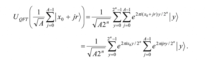
x = x0. Given that f(x + kr) = f(x), where r is the period of the function f and k is an integer, the first register will correspondingly attain a superposition of state vectors {…, x0-r, x0, x0+r, x0+2r,…}.. So, the state of the combined registers is

For notational convenience, we now choose x0 to be the lowest x∈{0,…, 2n-1} such that f(x) = f(x0). Thus, the index j in the summation will take the values 0, 1,…, A-1. We now apply the QFT to the first register
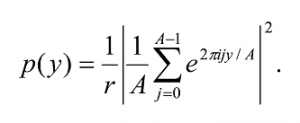
A measurement of the first register will yield a |yâ© with probability
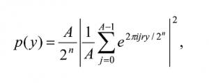
since
When r divides 2n exactly, A = 2n/r and A/ 2n = 1/r, the probability becomes
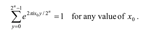
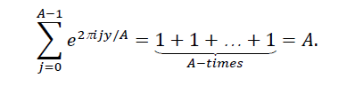
If y = A, 2A, etc., then
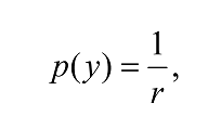
because jy/A is an integer and hence
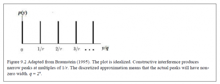
But if y is incommensurate (irrational) with A, then we will hit a range of points around the circle, eventually filling the whole circle so the resulting interference will be totally destructive, and we will have p(y) = 0. Therefore, in effect, the measurement will return a y ∈{A, 2A,…, rA}. From this we can easily find A, and knowing the range 2n we can find r = 2n/A.
In general, r will not divide 2n exactly, so measurements will return y scattered around integer multiples of 1/r, such that the constructive interferences produce narrow peaks at multiples of 1/r. Thus, we will obtain only a random multiple of the inverse period. To extract the period itself we will need to repeat this quantum computation roughly log log r/n times in order to have a high probability for at least one of the multiples to be relatively prime19 to the period r, thereby uniquely determining the period. This algorithm yields only a probabilistic answer but the probability can be made as high as we like. The actual determination of r can be made by using the continued fractions algorithm.
This is a method for determining for an arbitrary real number, x, an expansion of the form20
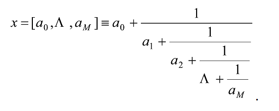
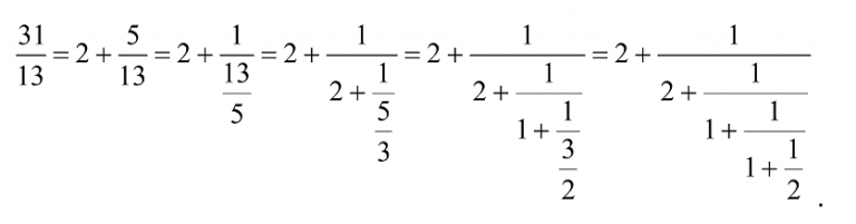
Consider, for example, 31/13. This is successively split into its integer and fractional parts,
A truncated continued fraction is called a convergent. The k-th convergent is written [a0,…, ak]. The decomposition terminates when the fraction has a numerator or a denominator of 1. The method terminates after a finite number of ‘split and invert’ steps for any rational number, since successive numerators are strictly decreasing.
One can show that if φ= s/r is a rational number and s and r are L bit integers, then the continued fraction expansion for φ can be computed using O(L3) operations—O(L) ‘split and invert steps’ and O(L2) gates for elementary arithmetic. There is also a useful theorem about continued fractions.
Theorem 1. If s/r is any rational number satisfying |s/r- φ| ≤ 1/(2r2) then s/r is a convergent of the continued fraction for φ . Moreover the convergent is such that gcd(s, r) = 1.
We can use this theorem to find the closest rationals to the terms s/r and hence find the period r. Furthermore, given φ the continued fractions algorithm efficiently produces numbers s’ and r’ with no common factor, such that s’/r’ = s/r. Euclid’s Algorithm for finding the greatest common divisor of two numbers is intimately related to continued fractions21.
To find the period, r, measure the state of the first register. This effectively samples from the discrete Fourier transform, and returns some number y’ that is some multiple s of q/r; that is y’ /q ≈ s/r for some positive integer s. To determine the period r we need to estimate s. This is accomplished by computing the continued fraction expansion for y’/q. By repeating the quantum computation several times (roughly log log r/n times) we create a set of samples of the discrete Fourier transform in the first register. This gives samples of multiples of 1/r as s1/r, s2/r, s3/r,… for various integers si. Once sufficient samples have been obtained from the first register, we can use the continued fraction technique to compute as to what the si could be and hence to guess r.
Computing the period of a sequence lies at the heart of efficiently factoring numbers, which we discuss below.
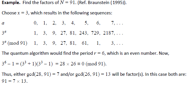
The problem of distinguishing prime numbers from composites, and of resolving composite numbers into their prime factors, is one of the most important and useful in all of arithmetic. […] The dignity of science seems to demand that every aid to the solution of such an elegant and celebrated problem be zealously cultivated. – Carl Friedrich Gauss
In 1994, Peter Shor surprised the world by describing a polynomial time quantum algorithm for factoring integers22. It was declared a killer application and received huge publicity because the widely used RSA23, a public key crypto-system, used in securing electronic bank accounts suddenly became utterly vulnerable. It relies on the difficulty of finding prime factors of large numbers. Shor’s algorithm was a shot in the arm to the quantum computing community.
Shor’s factoring algorithm has two parts: a quantum procedure within the algorithm and a classical algorithm that calls the quantum procedure. The algorithm uses a number theory result that relates the period of a particular periodic function to the factors of an integer. The crux of the algorithm is the quantum method for computing the period r of the function f(a) = xa mod N for a = 0, 1,… that is exponentially more efficient than any known classical method. Thus, given an integer N (the number to be factored), construct f(a) = xa mod N where x < N is a randomly chosen number which is coprime24 to N. It can be shown that f(a) thus constructed is periodic, that is,
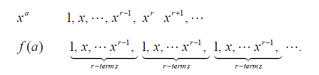
Here r is the first non-trivial power where xr ≡ 1 mod N, and that f(a) is periodic with period r, i.e., f(a) = f(a+r) = f(a+2r) = … Obviously, different values of x may produce different periodicities. The periodicity of f(a) can be determined by using the quantum algorithm described in Section 10.2. For a given N and a chosen x if the period r is an even number, we can write
19 Two integers are relatively prime if they do not share common positive factors (divisors) except 1.
20 For applications in quantum computing, it is convenient to allow a0 = 0 as well.
21 For a good description of continued fractions and an online calculator, see Knott ().
22 Shor (1994). An expanded version of the paper is available in Shor (1997).
23 The RSA system was invented by Ronald Rivest, Adi Shamir, and Leonard Adleman in 1978. It rules e-commerce and pops up in countless security applications. They received the Turing Award (2002) for their contributions to public key cryptography.
24 Coprime: Two integers a and b are coprime (or relatively prime) if the greatest common divisor of a and b is 1. For example, 55555 and 7811 are coprime even though neither number is itself a prime. One may use Euclid’s algorithm to determine if x and N are coprime.
in the alternative form
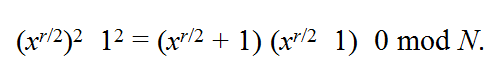
This implies that the product of the two factors on the left is a multiple of the number N. So, unless xr/2 ≡±1 mod N, at least one of these factors must be in common with N. Thus we have a good chance of finding a factor of N by computing, gcd(xr/2 + 1, N) and gcd(xr/2 – 1, N).
If r is odd, we choose another x and redo the previous steps till an x is found for which r is even. (With randomly chosen x, an even r will happen 50% of the time.) Once a factor u is found, Shor’s algorithm is repeated on N1 = N/u, and so on till all the factors of N are found.
The quantum part of Shor’s algorithm is determining the period r, and the classical part is computing the function gcd(), which is efficiently done using Euclid’s algorithm.
Shor’s algorithm verified. On Dec 19, 2001 IBM announced that it had built a 7-qubit quantum computer based on seven atoms which, because of the physical properties of those atoms, were able to work together as both the computer’s processor and memory, and that they were able to use the computer to show that Shor’s algorithm works by correctly identifying 3 and 5 as the factors of 1525.
Computational complexity of Shor’s algorithm. On classical computers (Turing machines) the best known factoring algorithm (the number field sieve) runs in O(exp[(64/9)1/3(ln N)1/3(ln ln N)2/3]) steps. This algorithm, therefore, scales exponentially with the input size log N. To give an example, in 1994, a 129-digit number was successfully factored using this algorithm on approximately 1600 workstations scattered around the world; the entire factorization took eight months. It was estimated that factoring a 250-digit number would take roughly 800,000 years and a 1000-digit number would require 1025 years (longer than the age of the universe!). Shor’s algorithm runs in O((log N)3) steps. This is roughly quadratic in the input size, so factoring a 250-digit number would require only a few billion steps.
In 1996, Lov Grover found an efficient quantum search algorithm for the problem: Given an unstructured list of N elements, find a specific element x0 in the list. Grover’s algorithm is much faster than any known classical algorithm26.
For convenience, each element is mapped to a unique index, which is just a number in the range 0 to N-1. Further, assume that N = 2n (the index can be stored in n bits) and that the search problem has exactly M solutions, with 1 ≤M ≤ N. A particular instance of the search problem can be conveniently represented by a function f, which takes an integer x as input in the range 0 to N-1. By definition, f(x) = 1 if x is a solution to the search problem, otherwise f(x) = 0.
We now introduce the notion of a quantum oracle – a black box unitary operator O. The oracle’s unique ability is to recognize solutions of the search problem. It does this by setting an oracle qubit |qâ© in the following manner
![]()
where |xâ© is the index register. We can check if x is a solution to our search problem by preparing |x, 0â©, applying the oracle, and checking to see if the oracle qubit has been flipped to |1â©. (Recall that a similar trick was used in the Deutsch problem.)
Here, instead, we apply the oracle with the oracle qubit initially in the state (|0â© – |1â©)/√2. If x is not a solution (i.e., f(x) = 0) to the search problem, applying the oracle to the state |x(|0â© -|1â©)/√2 does not change the state. But if x is a solution, then |0â© and |1â© get interchanged to give the final state as – |x(|0â© -|1â©)/√2. That is,
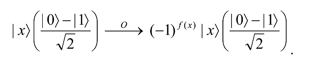
In this representation, the state of the oracle qubit has not changed; it remains (|0â© – |1â©)/√2 throughout the quantum search algorithm, and therefore can be omitted from further discussion! Hence it is customary to depict the action of the oracle as follows:
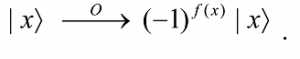
and to note that the oracle marks the solution to the search problem by shifting the phase of the solution. There is, however, a subtle point here. In the above operation, the oracle does not know the answer, it can only recognize the answer! It is, of course, possible to do the latter without being able to do the former. For example, finding the prime factors of a very large number is a known difficult problem. But if the prime factors are given, we can easily verify if their product is the given number. The point is that even without knowing the prime factors, one can explicitly construct an oracle, which recognises the factors when it sees one.
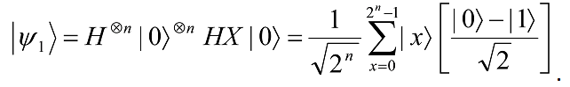
Grover’s search algorithm begins with an n-qubit register in the state |0â©⊕n, to which the Hadamard transform is applied and an oracle qubit in the state |0â© to which HX is applied:
To this we iteratively apply the Grover operator G, comprising the following 4 steps:
The oracle O marks solutions to the search problem by shifting the phase of the solution. Thus
where f(x) = 1 if x is a solution else f(x) = 0.
The third step requires a conditional phase shift to be applied to every computational basis state, except |0â©, such that, |0â© →|0â© and |xâ© → -|xâ© for x > 0. This is done by the operator 2|0â©â¨0|- I.
Thus, G is
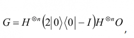
where the operator 2|0â©â¨0| – I flips states about the |0â© axis, i.e., it reverses every basis state except for |0â©. Further let |Ψâ©= H⊕n |0â©. Then since H2 = I, we can rewrite G as

One may show that the operation 2|Ψâ©â¨Ψ| – I applied to a general state

produces
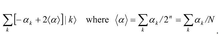
Here ⨠α â© is the mean value of the αk. For this reason, 2|Ψâ©â¨Ψ| – I is sometimes referred to as the inversion about the mean operation.
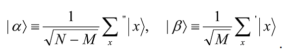
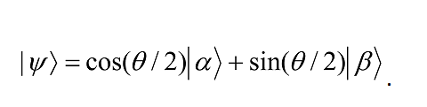
So, what does the Grover iteration do? Well, it can be seen as a rotation in the two-dimensional space spanned by the starting vector |Ψâ© and the state consisting of a uniform superposition of solutions to the search problem. To see this clearly, let the prime on the summation sigma symbol below indicate a sum over the M values of x which are solutions to the search problem, and the double prime on the summation sigma symbol a sum over the remaining N-M values of x. Define normalized states as follows:
Hence the initial state |Ψâ© may now be re-expressed as

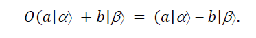
So, the initial state of the computer is in the space spanned by |αâ© and |βâ©. On this space the oracle O essentially performs a reflection about the vector |αâ© in the plane defined by |αâ© and |βâ©. That is,
Similarly, 2|Ψâ©â¨Ψ|- I also causes a reflection in the plane defined by |αâ© and |βâ© about the vector |Ψâ© . And the product of two reflections is a rotation! We notice two things here. First, after the k-th iteration, the state Gk |Ψâ© remains in the space spanned by |αâ© and |βâ© for all k. Second, it gives us the rotation angle. To get the rotation angle, let
![]()
so that
The two reflections that comprise G take |Ψâ© to
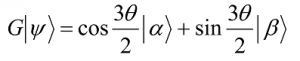
so the rotation angle is in fact θ. Repeated k applications of G takes the state to
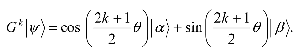
Thus, G produces a rotation in the two-dimensional space spanned by |αâ© and |βâ©, rotating the space by θ radians per application of G. Repeated application of G rotates the state vector close to |βâ©. After R iterations, an observation in the computational basis produces, with high probability, one of the outcomes superposed in |βâ©, i.e., a solution to the search problem.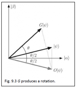
Thus, in the|αâ©, |βâ© basis, Grover’s iteration can be written as
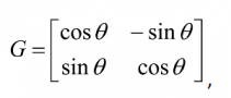
where θ is a real number in the range 0 to π/2.
How is R chosen? Note that the initial state of the system was
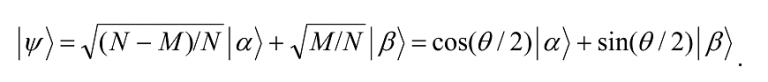
Hence |Ψâ© needs to be rotated by π/2 –θ/2 from its initial position to reach the solution state |βâ©. Note also that
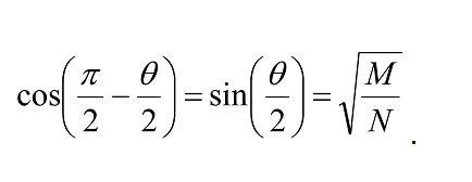
Therefore, rotating through
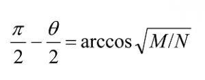
radians takes the system to |βâ© . Let CI(x) denote the integer nearest to the real number x, where by convention we round halves down – CI(3.5) = 3, for example – so that CI(x)≤ x. Then applying the Grover iteration
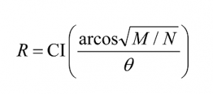
times rotates |Ψâ© to within an angle π/2 ≤π/4 of |βâ©. Observation of the state in the computational basis then yields a solution to the search problem with probability at least one-half. In fact, for specific values of M and N it is possible to achieve a much higher probability of success. For example, when M << N we have θ≈sin θ≈ 2√(M/N), and thus the angular error in the final state is at most θ/2≈ √(M/N), giving a probability of error of at most M/N. Note that R depends on the number of solutions M, but not on the identity of those solutions. Thus, applying Grover’s iteration, G, R times, for the case M = 1, we have
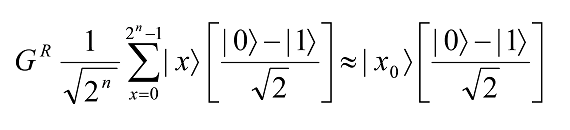
The result x0 is found by measuring the first n- qubits.
Boyer et al27 have shown that if there is a single solution x0, then after (π/8)√(2n) number of Grover iterations the failure rate is 0.5. After (π/4)√(2n) iterations the failure rate drops to 2-n. However, additional iterations will increase the failure rate! For example, after (π/2)√(2n) iterations the failure rate is close to 1. The reason is that unitary transformations are rotations in complex space, and thus while a repeated application of a quantum transformation may rotate the state closer and closer to the desired state for a while, eventually it will rotate past that state and get farther and farther away. Thus, to obtain useful results from a repeated application of a quantum transformation, one must know when to stop.
26 Grover (1997a). See also: Grover (1997b). A popularized version of the algorithm appears in Grover (1999).
27 Boyer, et al (1996).
28 See Chuang, Gershenfeld & Kubinec (1998). See also: Gershenfeld & Chuang (1998).
Grover’s algorithm verified. In 1997, Isaac L. Chuang (IBM, Almaden), Neil A. Gershenfeld (MIT, Cambridge), and Mark G. Kubinec (Univ. of California, Berkeley) actually built a simple two-qubit NMR quantum computer using liquid chloroform (CHCl3) and successfully ran Grover’s algorithm28. In 2000, Chuang and his team reported the experimental implementation of Grover’s algorithm on a three-qubit NMR quantum computer comprising molecules of 13C-labeled CHFBr2, in which the three weakly coupled spin-1/2 nuclei behave as the bits and are initialized, manipulated, and read out using magnetic resonance techniques29.
Computational complexity of Grover’s algorithm. It is well known that classical methods for this search problem require n/2 searches on average to find a solution. Grover’s algorithm requires O√(n) steps. Not only that, Grover’s algorithm is also the fastest even among all possible quantum algorithms for this problem30. Note that the task remains computationally hard, that is, it is not transferred to a new complexity class, but it is remarkable that such a seemingly hopeless task can be speeded up at all. Any problem for which finding solutions is hard, but testing a candidate solution is easy, can as a last resort be solved by an exhaustive search. In such cases, Grover’s algorithm may prove very useful.
Remarks on Grover’s algorithm. There are variations of Grover’s algorithm, which can find the largest or smallest value in a list, or the modal value31, and so on. So, it is quite a versatile searching tool. However, in practice, searching a physical database is unlikely to become a major application of Grover’s algorithm for non-algorithmic reasons, at least so long as classical memory remains cheaper than quantum memory. For since the operation of transferring a database from classical to quantum memory (bits to qubits) would itself require O(n) steps, Grover’s algorithm would improve search times by at best a constant factor, which could also be achieved by classical parallel processing. Grover’s algorithm becomes really useful when searching through lists that are not stored in memory but are themselves generated on the fly by a computer program.
Bennett and Wiesner32 found a method that uses an entangled pair of qubits to encode and transmit two classical bits worth of information. Since entangled pairs can be distributed ahead of time, only one qubit needs to be physically transmitted from sender to receiver to communicate two bits of information. Hence the name dense coding.
If Alice and Bob wish to communicate in this manner, then each is sent one particle from an entangled pair of particles in the state33
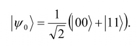
Let Alice get the first particle and Bob the second. The distribution of the entangled particles between the two establishes a quantum communication channel between them. Note that there are four mutually orthogonal states |00â© + |11â©, |00â©- |11â©, |01â© + |10â©, |01â© -|10â©, which form the Bell basis. So, when, Alice receives two classical bits, encoding the numbers 0 through 3, she performs one of the following transformations on her qubit depending on the encoded number:
29 Vandersypen, et al (2000).
30 Bennett, et al (1997).
31 Modal value: the most frequently occurring value.
32 See Bennett & Wiesner (1992). See also: Rieffel & Polak (2000).
33 See, e.g., Rieffel & Polak (2000).
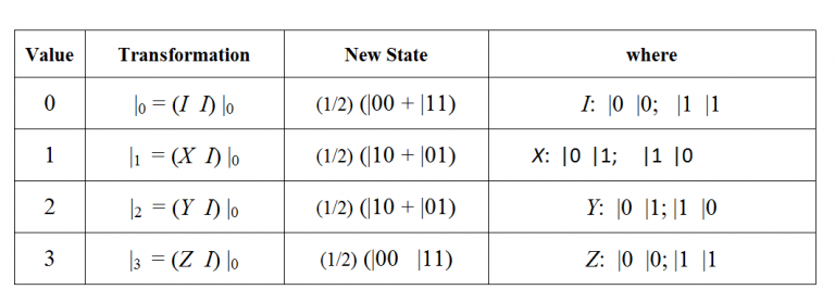
Since there are four possibilities, her choice of operation represents two bits of classical information. Note that transforming just one bit of an entangled pair means performing the identity transformation on the other bit. Alice then sends her qubit to Bob who must deduce which Bell basis state the qubits are in. Bob first applies a controlled-NOT to the two qubits of the entangled pair.
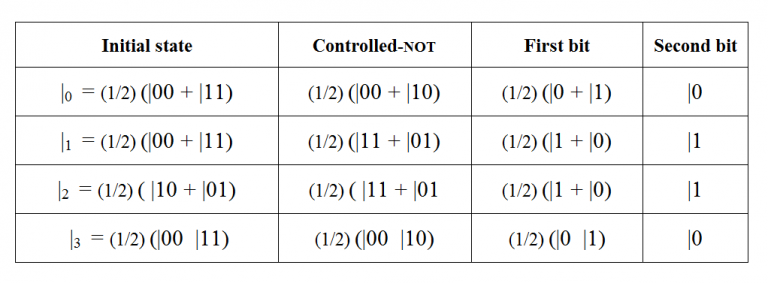
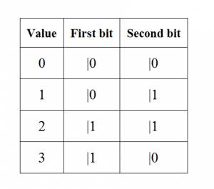
Bob then measures the second qubit. If the measurement returns |0â©, the encoded value was either 0 or 3; otherwise the value was either 1 or 2. Bob now applies H to the first bit and measures that bit (see Table below).
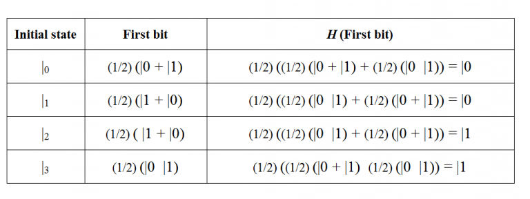
This allows him to distinguish between 0 and 3, and 1 and 2, as shown in the table below.
In principle, dense coding can permit secure communication: the qubit sent by Alice will only yield the two classical information bits to someone in possession of the entangled partner qubit. But more importantly, it shows why quantum entanglement is an information resource. It reveals a relationship between classical information, qubits, and the information content of quantum entanglement.
Teleportation is the ability to transmit the quantum state of a given particle using classical bits and to reconstruct that exact quantum state at the receiver. The no-cloning principle, however, requires that the quantum state of the given particle be necessarily destroyed. Instinctively, one perhaps realizes that teleportation may be realizable by manipulating a pair of entangled particles; if we could impose a specific quantum state on one member of an entangled pair of particles, then we would be instantly imposing a predetermined quantum state on the other member of the entangled pair. The teleportation algorithm is due to Charles Bennett and his team (1993)34.
Teleportation of a laser beam consisting of millions of photons was achieved in 1998. In June 2002, an Australian team reported a more robust method of teleporting a laser beam. Teleportation of trapped ions was reported in 200435. In May 2010, a Chinese research group reported that they were able to “teleport” information 16 kilometers36. In July 2017, a Chinese team reported “the first quantum teleportation of independent single-photon qubits from a ground observatory to a low Earth orbit satellite – through an up-link channel – with a distance up to 1400 km”37. This experiment is an important step forward in establishing a global scale quantum internet in the future. In theory, there is no distance limit over which teleportation can be done. But since entanglement is a fragile thing, there are technological hurdles to be overcome.
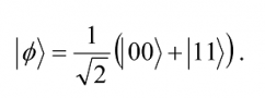
To see how teleportation works, let Alice possess a qubit of unknown state |Øâ© = a |0â© + b |1â©. She wishes to send the state of this qubit to Bob through classical channels. In addition, Alice and Bob each possess one qubit of an entangled pair in the state
Alice applies the decoding step of dense coding to the qubit ∅ to be transmitted and her half of the entangled pair. The initial state is
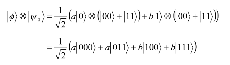
of which Alice controls the first two qubits and Bob controls the last qubit. She now applies Cnot⊗ I and H⊗ I⊗ I to this state:
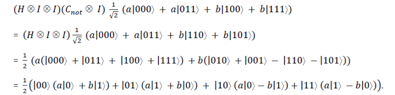
Alice measures in the Bell basis the first two qubit to get one of |00â©, |01â©, |10â©, or |11â© with equal probability. That is, Alice’s measurements collapse the state onto one of four different possibilities, and yield two classical bits. Alice sends the result of her measurement as two classical bits to Bob. Depending on the result of the measurement, the quantum state of Bob’s qubit is projected to a(|0â© + b|1â©, a(|1â© + b|0â©, a(|0â©- b|1â©, or a(|1â© -b|0â© respectively38. Note that Alice’s measurement has irretrievably altered the state of her original qubit ∅ , whose state she is trying to send to Bob. Thus, the no-cloning principle is not violated. Also, Bob’s particle has been put into a definite state.
When Bob receives the two classical bits from Alice he knows how the state of his half of the entangled pair compares to the original state of Alice’s qubit.
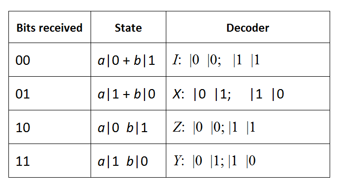
Bob can reconstruct the original state of Alice’s qubit ∅ by applying the appropriate decoder to his part of the entangled pair. Note that this is the encoding step of dense coding.
The interesting facts to note are as follows. First, the state that is transmitted is completely arbitrary (not chosen by Alice and unknown to her). Second, a message with only binary classical information, such as the result of the combined experiment made by Alice is definitely not sufficient information to reconstruct a quantum state; in fact, a quantum state depends on continuous parameters, while results of experiments correspond to discrete information only. Somehow, in the teleportation process, binary information has turned into continuous information! The latter, in classical information theory, would correspond to an infinite number of bits.
It also happens that Alice cannot determine the state of her particle with state ∅ by making a measurement and communicating the result to Bob because it is impossible to determine the unknown quantum state of a single particle (even if one accepts only an a posteriori determination of a perturbed state); one quantum measurement clearly does not provide sufficient information to reconstruct the whole state, and several measurements will not provide more information, since the first measurement has already collapsed the state of the particle. Note also that without the classical communication step, teleportation does not convey any information at all. The original qubit ends up in one of the computational basis states |0â© or |1â© depending on the measurement outcome.
Quantum teleportation can be used to move quantum states around, e.g., to shunt information around inside a quantum computer or indeed between quantum computers. Quantum information can be transferred with perfect fidelity, but in the process the original must be destroyed. This might be especially useful if some qubit needs to be kept secret. Using quantum teleportation, a qubit could be passed around without ever being transmitted over an insecure channel. In addition, teleportation inside a quantum computer can be used as a security feature wherein only one version of sensitive data is ensured to exist at any one time in the machine. We need not worry about the original message being stolen after it has been teleported because it no longer exists at the source location. Furthermore, any eavesdropper would have to steal both the entangled particle and the classical particle in order to have any chance of capturing the information.
Thus far we have, by a variety of examples, shown the power of quantum computing. In Section 10 we concluded Part II by describing some of the prized algorithms.
Readers desirous of getting some hands-on experience with a few of the algorithms presented in Part II can visit https://acc.digital/Quantum_Algorithms/Quantum_Algorithms_June2018.zip . This material is provided by Vikram Menon using the IBM Q Experience for Researchers (see https://quantumexperience.ng.bluemix.net/qx/experience).
34 Bennett, et al (1993). See also: Rieffel & Polak (2000).
35 Riebe, et al (2004). Barrett, et al (2004).
36 Jin, et al (2010).
37 Ren, et al (2017). A report appears in: Emerging Technology from the arXiv. First Object Teleported from Earth to Orbit. MIT Technology Review, 10 July 2017, https://www.technologyreview.com/s/608252/first-object-teleported-from-earthto- orbit of the states a(|0â© + b|1â©, a(|1â© + b|0â©, a(|0â©- b|1â©, or a(|1â© – b|0â©.
38 Note that due to the measurement Alice made, the measured qubits have collapsed. Hence only Bob’s qubit can be in one
Cited URLs were last accessed on 31 January 2018.
Allenby & Redfern (1989). Allenby, R. B. J. T., and Redfern, E. J. Introduction to Number Theory with Computing. Edward Arnold, London, 1989.
Baeyer (2001). von Baeyer, H. C. Tangled Tales. The Sciences, Spring, 2001.
Barenco (1996). Barenco, A., Quantum Physics and Computers. Contemporary Physics, 37, 375-389, 1996.
Barrett, et al (2004). Barrett, M. D., Chiaverini, J., Schaetz, T., Britton, J., Itano, W. M., Jost, J. D., Knill, E., Langer, C., Leibfried, D., Ozeri, R., and Wineland, D. J. Deterministic Quantum Teleportation of Atomic Qubits. Nature, Vol. 429, 737-739, 17 June 2004. http://www.boulder.nist.gov/timefreq/general/pdf/1926.pdf
Bennett (1992). Bennett, C. H. Quantum Cryptography Using any Two Nonorthogonal States. Physical Review Letters, 68, 3121-3124, 1992.
Bennett (1994). Bennett, C. H. Interferometric Quantum Cryptographic Key Distribution System. US Patent No. US5307410, 26 April 1994. https://patentimages.storage.googleapis.com/pdfs/US5307410.pdf
Bennett & Brassard (1984). Bennett, C. H., and Brassard, G. Quantum Cryptography: Public Key Distribution and Coin Tossing. Proceedings of IEEE International Conference on Computers, Systems and Signal Processing, 175-179. IEEE, New York, 1984. http://www.research.ibm.com/people/b/bennetc/bennettc198469790513.pdf
Bennett & Brassard (1989). Bennett, C. H., and Brassard, G. The Dawn of a New Era for Quantum Cryptography: The Experimental Prototype is Working! SIGACT News, 20, 78-82, Fall 1989.
Bennett, et al (1993). Bennett, C. H., Brassard, G., Crépeau, C., Jozsa, R., Peres, A., and Wootters, W. K. Teleporting an Unknown Quantum State via Dual Classical and Einstein–Podolsky–Rosen Channels, Physical Review Letters, 70 (13), 1895–1899, 1993. https://www.research.ibm.com/people/b/bennetc/BBCJPW.pdf
Bennett, et al (1997). Bennett, C.H., Bernstein, E., Brassard, G., and Vazirani, U. Strengths and Weaknesses of Quantum Computing. Preprint quant-ph/9701001, 1997. https://arxiv.org/pdf/quant-ph/9701001.pdf
Bennett & Wiesner (1992). Bennett, C. H., and Wiesner, S. J. Communication via One- and Two-Particle Operators on Einstein-Podolsky-Rosen States. Physical Review Letters, 69 (20), 2881-2884, 1992.
Bennett & Wiesner (1996). Bennett, C. H., and Wiesner, S. J. Quantum Key Distribution Using Non-Orthogonal Macroscopic Signals. US Patent No. US5515438, 07 May 1996. https://docs.google.com/viewer?url=patentimages.storage.googleapis.com/pdfs/US5515438.pdf
Black, Kuhn & Williams (2002). Black, P. E., Kuhn, D. R., and Williams, C. J. Quantum Computing and Communications. In Advances in Computers, Marvin Zelkowitz (Ed.), 56, 189-244, 2002. Preprint at https://pdfs.semanticscholar.org/db97/6452bc9388b9df3c9ea6b5c8228041dde395.pdf
Boyer, et al (1996). Boyer, M., Brassard, G., Hoyer, P., and Tapp, A. Tight Bounds on Quantum Search. Proceedings of the Workshop on Physics of Computation: PhysComp ’96, Los Alamitos, CA, 36-43, 1996. http://xxx.lanl.gov/abs/quant-ph/9805082
Braunstein (1995). Braunstein, S. L.. Quantum Computation. 1995. http://www-users.cs.york.ac.uk/~schmuel/comp/comp_best.pdf
Chuang, Gershenfeld & Kubinec (1998). Chuang, I.L., Gershenfeld, N., and Kubinec, M. Experimental Implementation of Fast Quantum Searching. Physical Review Letters, 80, 3408–3411, 1998.
Cleve, et al (1998). Cleve, R., Ekert, A., Macchiavllo, C., and Mosca, M., Quantum Algorithms Revisited. Proceedings of the Royal Society of London, Series A, , Mathematical, Physical and Engineering Sciences, 454 (1969), 339-354, 1998. See preprint at: arXiv:quant-ph/9708016 v1 8 Aug 1997, http://arxiv.org/PS_cache/quant-ph/pdf/9708/9708016v1.pdf.
Coppersmith (1994). Coppersmith, D. An Approximate Fourier Transform Useful in Quantum Factoring. IBM Research Report RC 19642 (1994).
Deutsch (1985). Deutsch, D. Quantum Theory, the Church-Turing Principle and the Universal Quantum Computer. Proceedings of the Royal Society of London; Series A, Mathematical and Physical Sciences, 400 (1818), 97–117, 1985. http://www.qubit.org/oldsite/resource/deutsch85.pdf.
Deutsch (1994). Deutsch (1994). Deutsch, D. Unpublished.
Deutsch & Jozsa (1992). Deutsch, D., and Jozsa, R. Rapid Solutions of Problems by Quantum Computation. Proceedings of the Royal Society of London A, 439, 553 -558, 1992. http://www.qudev.ethz.ch/phys4/studentspresentations/djalgo/DeutschJozsa.pdf
DeWeerd (2002). DeWeerd, A. J. Interaction-Free Measurement. American Journal of Physics, 70 (3), March 2002. https://www.redlands.edu/contentassets/e8193043b14545aca28afd326b500d3d/ifm-ajp.pdf
Ekert & Jozsa (1996). Ekert, A., and Jozsa, R. Quantum Computation and Shor’s Factoring Algorithm. Reviews of Modern Physics, 68 (3), 733-753, 1996. http://citeseerx.ist.psu.edu/viewdoc/download?doi=10.1.1.173.1518&rep=rep1&type=pdf
Elitzur & Vaidman (1993). Elitzur A. C. and Vaidman L. Quantum Mechanical Interaction-Free Measurements. Foundations of Physics, 23, 987-97, 1993. Preprint at http://arxiv.org/PS_cache/hep-th/pdf/9305/9305002v2.pdf
Gershenfeld & Chuang (1998). Gershenfeld, N. A., and Chuang, I.L. Quantum Computing with Molecules. Scientific American, 278 (6), 66-71, June 1998. http://cba.mit.edu/docs/papers/98.06.sciqc.pdf
Goldreich (2004). Goldreich, O. Foundations of Cryptography, 2. Cambridge University Press, 2004. http://www.wisdom.weizmann.ac.il/~oded/foc-book.html
Grover (1997a). Grover, L. K. A Fast Quantum Mechanical Algorithm for Database Search. Proceedings of the 28th Annual ACM Symposium on the Theory of Computing, Philadelphia, 212-219, 1996. Available at http://xxx.lanl.gov/abs/quant-ph/9605043
Grover (1997b). Grover, L. K. Quantum Mechanics Helps in Searching for a Needle in a Haystack. Physical Review Letters, 79 (2), 325-328, 14 July 1997. Available at https://arxiv.org/pdf/quant-ph/9706033.pdf
Grover (1999). Grover, L. K. Quantum Computing. The Sciences, 24-30, July/August 1999. http://cryptome.org/qc-grover.htm
Jin, et al (2010). Jin, X-M., et al, Experimental Free-Space Quantum Teleportation. Nature Photonics, 4, 376-381, 2010, Published online: 16 May 2010.
Knott (). (). Knott, R. Fibonacci Numbers and the Golden Section. http://www.maths.surrey.ac.uk/hosted-sites/R.Knott/Fibonacci/cfINTRO.html
Kwiat, et al (1995a). Kwiat, P., Weinfurter, H., Herzog, T., Zeilinger, A., and Kasevich, M. Interaction-Free Measurement. Physical Review Letters, 74 (24), 4763-4766, 1995. http://research.physics.illinois.edu/QI/Photonics/papers/My%20Collection.Data/PDF/Interaction-Free%20Measurement.pdf
Kwiat, et al (1995b). Kwiat, P., Weinfurter, H., Herzog, T., Zeilinger, A., and Kasevich, M. Experimental Realization of Interaction-free Measurements. Fundamental Problems in Quantum Theory: A conference held in honor of Professor John A. Wheeler. Annals of the New York Academy of Sciences, 755, 383-393, 07 April 1995. The conference was sponsored by the New York Academy of Sciences and held on June 18-22, 1994, in Baltimore, Maryland.
Kwiat, et al (1995c). Kwiat, P., Weinfurter, H., Herzog, T., Zeilinger, A., and Kasevich, M. Experimental Realization of “Interaction-Free” Measurements. Quantum Electronics and Laser Science Conference OSA Technical Digest (Optical Society of America, 1995), paper QTuF5, 1995. A version available at http://www.univie.ac.at/qfp/publications3/pdffiles/1994-08.pdf
Penrose (1994). Penrose, R. Shadows of the Mind. Oxford University Press, 1994 (Vintage paperback).
Ren, et al (2017). Ren, J-G, et al. Ground-to-Satellite Quantum Teleportation. arXiv 1707.00934, 04 July 2017, https://arxiv.org/ftp/arxiv/papers/1707/1707.00934.pdf (paper) and https://arxiv.org/abs/1707.00934 (abstract)
Riebe, et al (2004). Riebe, M., Häffner, H., Roos, C. F., Hänsel, W., Benhelm, J., Lancaster, G. P. T., Körber, T. W., Becher, C., Schmidt-Kaler, F., James, D. F. V., and Blatt, R. Deterministic Quantum-Teleportation with Atoms. Nature, 429, 734-737, 17 June 2004. http://heart-c704.uibk.ac.at/Papers/Nature04_Riebe.pdf, see also http://heart-c704.uibk.ac.at/RecentResults/QuantumTeleportationE.html.
Rieffel & Polak (2000). Rieffel, E., and Polak, W. An Introduction to Quantum Computing for Non-Physicists, ACM Computing Surveys. 32 (3), 300-335, September 2000. An earlier version available at https://arxiv.org/pdf/quant-ph/9809016.pdf
Rivest, Shamir & Adleman (1978). Rivest, R. L., Shamir, A., and Adleman, L. M. A Method of Obtaining Digital Signatures and Public-key Cryptosystems. Communications of the ACM, 21 (2), 120-126, 1978. Available at https://people.csail.mit.edu/rivest/Rsapaper.pdf
Shor (1994). Shor, P. W. Algorithms for Quantum Computation: Discrete Log and Factoring. Proceedings of the 35th Annual Symposium on Foundations of Computer Science, 124-134, November 1994. ftp://netlib.att.com/netlib/att/math/shorquantum.algorithms.ps.Z
Shor (1997). Shor, P. W. Polynomial-Time Algorithms for Prime Factorization and Discrete Logarithms on a Quantum Computer. SIAM Journal on Scientific and Statistical Computing, 26 (5), 1484-1509, 1997. Preprint at http://www.arxiv.org/PS_cache/quant-ph/pdf/9508/9508027.pdf
Shor & Preskill (2000). Shor, P. W., and Preskill, J. Simple Proof of Security of the BB84 Quantum Key Distribution Protocol. Physical Review Letters, 85, 441-444, 2000. Available at arXiv:quant-ph/0003004v2
Vandersypen, et al (2000). Vandersypen, L. M. K., Steffen, M., Sherwood, M.H., Yannoni, C. S., Breyta, G., Chuang, I.L. Implementation of a Three-Quantum-Bit Search Algorithm. Applied Physics Letters, 76 (5), 646-648, 31 January, 2000. Available at https://arxiv.org/pdf/quant-ph/9910075.pdf
Vandersypen, et al (2001). Vandersypen, L. M. K., Steffen, M., Breyta, G., Yannoni, C. S., Sherwood, M. H., and Chuang, I. L. Experimental Realization of Shor’s Quantum Factoring Algorithm Using Nuclear Magnetic Resonance. Nature, 414, 883-887, 20-27 December 2001. http://www.fisica.uniud.it/~giannozz/Corsi/FisMod/Testi/nature.pdf
To be continued in Part III – The measurement conundrum
Linear Algebra
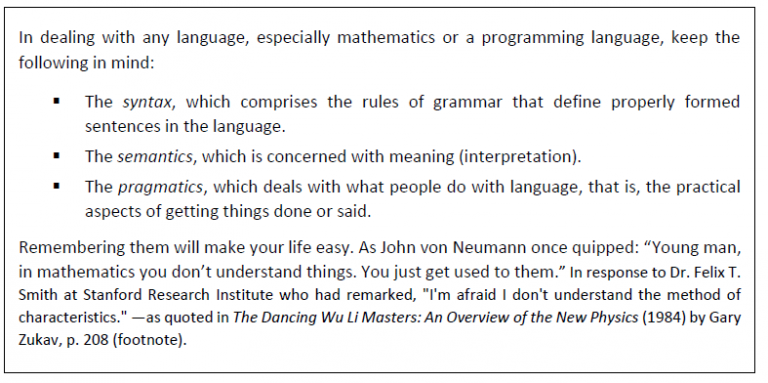
The basic objects in the study of linear algebra are vector spaces, in particular, the space Cn, of all n-tuples of complex numbers, (z1,…, zn). The elements of a vector space are called vectors. Physicists sometimes refer to complex numbers as c-numbers. The most familiar notation for a state vector in describing a quantum system is |Ψâ©. (Physicists can be rather flippant in their choice of symbols other than Ψ , e.g., +,- ,↑ , ↓, etc.) The standard vector-matrix notation is used when the state vector is expressed in terms of its components. For example,
Like ordinary vectors, state vectors are specified by a particular choice of basis vectors (eigenstates) and a particular set of complex numbers, corresponding to the amplitudes with which each eigenstate contributes to the complete state vector. Once the state vector |Ψâ© of a quantum system is known, the expected value of any observable attribute of the system can be calculated since |Ψâ© contains the complete information about the system. This is similar to descriptions of systems in classical physics in which the complete state of the system is known once the time-dependent functions for position and momentum are determined.
In what follows, it is advisable to pay attention to minute details of notation and syntax. Heed von Neumann’s observation and get used to them! Pay particular attention to all those mathematical properties which remain invariant under a given transformation, especially unitary transformations. Under unitary transformations, state vectors only rotate, they do not change length. We have generally stayed with the notations and manner of presentation of results provided in the excellent text book by Nielsen and Chuang39. This will also facilitate readers in going back and forth between this paper and the book by Nielsen and Chuang. The notations have a certain elegance.
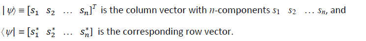
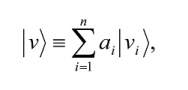
A vector |vâ© having n vector components |v1â©,…|vnâ© is generally written as the linear summation
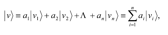
where a1, a2, … , an are n complex constants. It is customary to represent |vâ© in the following alternative matrix forms, if it is apparent from the context that |vâ© has the components |v1â©,…|vnâ©:
Note that in this notation, the matrix representation of |viâ© will have all ak = 0 for k = 1,…, n except for k = i, for which ai = 1. For example,|v3â© has the matrix representation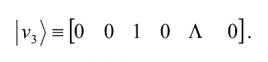
Note that when we use matrix notation to describe state transformations, the ordering of the basis vectors in the matrix representation must be settled a priori so that we can keep track of how each basis vector is transforming when it undergoes a transformation. Finally, when the context is clear in this paper, the abstract index form is also used for an abstract linear transformation or a set of basis vectors. For example, |iâ© may either stand for itself or for the basis set of which it is member.
A set of vectors |v1â© ,… |vnâ© is said to be a spanning set for a vector space V if any vector |vâ© in V can be written as a linear combination
where, for the given |vâ©, the complex coefficients ai are unique. Such a vector space V is said to have n dimensions, a fact symbolically stated by Cn.
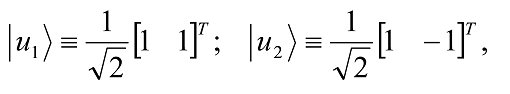
An example of a spanning set for the vector space C2 is the set
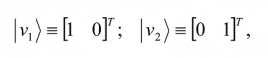
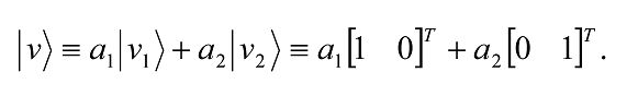
since any vector |vâ©≡ [a1 a2]T in C2 can be written as the following linear combination
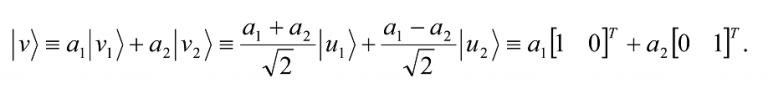
A vector space may have many different spanning sets. For example, a second spanning set for the vector space C2 is the set
as once again, any vector |vâ© [a1 a2]T in C2 can be written as the linear combination
A set of non-zero vectors |v1â©,… |vnâ© is said to be linearly dependent if there exists a set of complex numbers |a1â©,… |anâ© with ai ≠ 0 for at least one value of i, such that
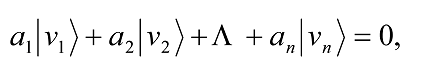
otherwise it is linearly independent. A linearly independent set is called a basis for V, and such a basis set always exists. The number of elements n in the basis is defined to be the dimension of V. Any two sets of linearly independent vectors, which span a vector space V, contain the same number n of elements.
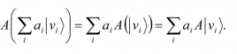
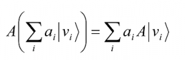
A linear operator between vector spaces V and W, where |v1â©,… |vmâ© is a basis for V and |w1â©,… |wnâ© is a basis for W (note that m and n may be different), is defined to be any function A: V → W, which is linear in its inputs40,
A linear operator A is said to be defined on a vector space V if A is a linear operator from V to V. The identity operator IV on a vector space V is defined by the equation IV |vâ© ≡ |vâ© for all vectors |vâ©. If the context is clear, IV is often abbreviated to I. In addition, there is a zero-operator denoted by 0, which maps all vectors to the zero vector, i.e., 0|vâ© ≡ 0. Note that the ket notation for the zero vector is not used as, by convention, it is reserved for the zero vector |0â© in quantum computing where it means something entirely different.
Sometimes it is easier to see linear operators in terms of their equivalent matrix representation. The claim that the matrix A is a linear operator simply means that
is true as an equation where the operation is matrix multiplication of
A by column vectors. The linear operator’s matrix representation is given by
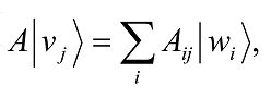
for each j in the range 1,… , m and an Aij is an element of A when represented in matrix form. The matrix representation of A is completely equivalent to the operator A. However, to make the connection between matrices and linear operators we must specify a set of input and output basis states for the input and output vector spaces, namely, V and W, respectively, of the linear operator A.
40 A: V → W means that A is a mapping from V to W, i.e., the input to A is V and the output of A is W. The space V is called the domain of A, and W the codomain of A. The range of A is the space Y = {y | y ∈ W and y = Ax for some x ∈ V}.
Three kinds of products between a pair of vectors |vâ© and |wâ© are defined. These are: inner product, outer product, and tensor product.
A.5.1 Inner product
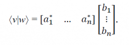
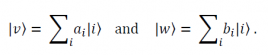
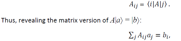
The inner product of |vâ© and |wâ© in the same vector space is represented by ⨠v|w â©. Let
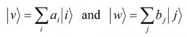
written with respect to the same orthonormal basis (this is a good time to get used to the abbreviated representation of vector components represented by their indices i and j such as |i â© for |viâ© and |j â© for |wj â© as done here, if the context is clear) with respect to some orthonormal basis of which |i is a member (this means that â¨i|jâ© = δij where δij = 1 if i = j else δij = 0; this can always be done by suitably adjusting the values of ai and bj depending on how the basis |iâ© is constructed. Several construction methods exist, a popular one being the Gram-Schmidt procedure) .Then
Since we can multiply any state vector by a non-zero complex number without changing its physical interpretation, we can always normalize the state so that it has unit length to make it a unit vector or put it, so to say, in a normalized state.
Note also that the inner product remains unaffected if each of the two vectors in the product is multiplied by the factor exp(iθ) (or its conjugate as applicable), where θ is real:
![]()
A.5.2 Outer product
The outer product
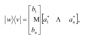
results in a n×n matrix. It is a useful way of representing linear operators. Moreover, the expression ⨠|wâ©â¨v|v’â© can be freely given any one of two meanings: (1) to denote the result when the operator |wâ©â¨v| acts on |v’â©; and (2) to denote the result of multiplying |wâ© by the complex number⨠v|v’â© . Mathematicians usually try to construct such clever symbolic systems for ease of manipulation and economy of expression when equivalences exist. One also notices that
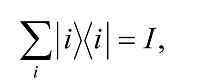
where the set of vectors represented by |iâ© is an orthonormal basis (i.e., ⨠i|jâ© = δij ) so that ⨠i|vâ© = ai and I is a n×n unit matrix. This equation is known as the completeness relation. By complete we mean that any state vector in the chosen vector space can be represented as a weighted sum of just the |iâ© vectors, e.g.,
For example, suppose A: V → W, is a linear operator, |viâ© is an orthonormal basis for V, and |wjâ© an orthonormal basis for W. Assume41
![]()
Now apply â¨i| to the above equations:
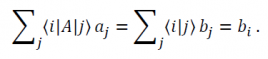
This allows us to extract any element of A with indices i, j be defining
A.5.3 Diagonal representation of an operator or orthonormal decomposition
A diagonal representation for an operator A on a vector space V is a representation
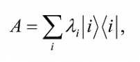
where the vectors |iâ© form an orthonormal set of eigenvectors for A, with corresponding eigenvalues λi. The i-th diagonal element of A is λi and all non-diagonal elements of A are zero. An operator which has a diagonal representation is said to be diagonalizable. Diagonal representations are also known as orthonormal decompositions. A diagonal representation of A simplifies computations tremendously since one need deal with only n elements of A rather than n2 elements for a n×n representation of A. So, an immediate computational advantage of knowing the eigenvalues and eigenvectors of an operator A is quite obvious. If all the eigenvalues of A are distinct, they can be used to index its eigenvectors.
41 B. Zwiebach, Dirac’s bra and ket notation, 8.05 Quantum Physics II, MIT OpenCourseWare, Fall 2013, 07 October 2013. https://ocw.mit.edu/courses/physics/8-05-quantum-physics-ii-fall-2013/lecture-notes/MIT8_05F13_Chap_04.pdf
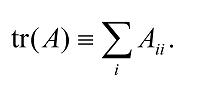
A.5.4 Trace of a matrix
Another important matrix function is the trace of a matrix, tr(A), defined as the sum of the diagonal elements of A (which need not be a diagonal matrix),
The trace is easily seen to be cyclic, that is, tr(AB) = tr(BA), and linear, i.e., tr(A + B) = tr(A) + tr(B), tr(zA) = z tr(A), where A and B are arbitrary matrices, and z is a complex number. It also follows from the cyclic property that the trace of a matrix is invariant under the unitary similarity transformation, A→UA† , since
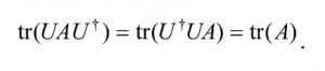
We define the trace of an operator A to be the trace of any matrix representation of A. The invariance of the trace under unitary similarity transformations ensures that the trace of an operator is well defined. It also means that if we choose a unitary transformation that diagonalizes A, then tr(?) = Σ? λi,i.e., the trace of A is also the sum of its eigenvalues, λi.
An extremely important formula (presented here without proof) for evaluating tr(A|Ψâ©â¨Ψ|) , where |Ψâ© is a unit vector and A is an arbitrary operator, is
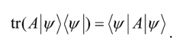
This result is extremely useful in evaluating the trace of an operator. It also plays a crucial role in deciding the probability with which a quantum system will collapse to a particular state when that system is measured. If A is the identity operator, then tr(|Ψâ©â¨Ψ| = â¨Ψ|Ψâ©).
A.5.5 Commutator and anti-commutator
The commutator between two operators A and B is defined as
[A, B] ≡ AB – BA.
If [A, B] = 0, that is, AB = BA, then we say A commutes with B. Similarly, the anti-commutator of two operators is defined by
{A, B} ≡ AB + BA.
A is said to anti-commute with B if {A, B} = 0. It so happens that many important properties of pairs of operators can be deduced from their commutator and anti-commutator. One such is the simultaneous diagonalization theorem, which states that if A and B are Hermitian operators, then [A, B] = 0 if and only if there exists an orthonormal basis such that both A and B are diagonal with respect to that basis. Thus, A and B are simultaneously diagonalizable in this case. It turns out that non-zero commutators play an essential role in the famous Heisenberg’s uncertainty principle in quantum mechanics. Indeed, non-commuting operators lie at the heart of quantum mechanics.
A.5.6 Tensor product
The tensor product of |vâ© and |wâ©, represented by |vâ©⊗ |wâ© (alternatively, by |vâ© |wâ© or |v , wâ© or |vwâ©), produces a matrix. The tensor product puts vector spaces together to form larger vector spaces. This simple method is crucial for constructing the Hilbert space for multi-qubit systems. Let A be a m×n matrix, and B a p×q matrix. Then the way vector spaces are put together is as follows:
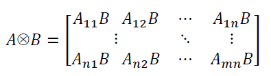
Here each element AijB represents a p×q submatrix whose entries are the entries of B multiplied by Aij. The fully expanded matrix form of A⊗B is a larger mp×nq matrix.
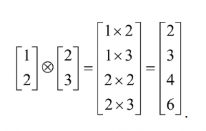
Example 1.
Finally, we have the useful notation |v⊗kâ© , which stands for |vâ© tensored with itself k times. For example,
By definition,
We shall shortly see that an analogous notation is used for operators (as they also have a matrix representation) on tensor product spaces.
By definition, the tensor product satisfies the following basic properties:
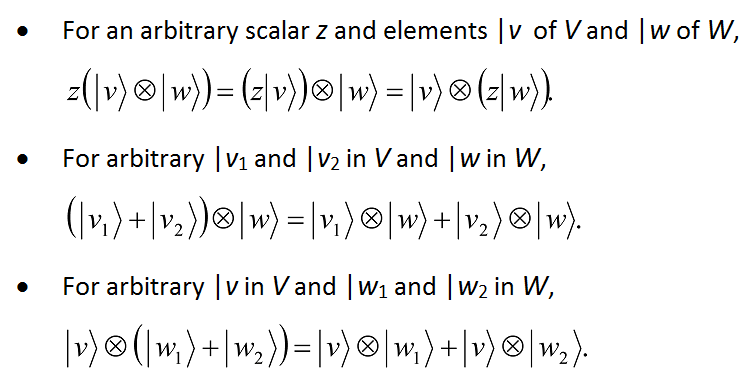
One may also show that

where the superscripts *, T, and †, respectively, denote complex conjugate, transpose, and Hermitian conjugate42 (or adjoint) operations on the entity they operate on.
Finally, we come to the nature of linear operators that act on the space |Vâ©⊗|Wâ©. By convention (and this is important), a matrix representation of a linear operator will imply that the representation is with respect to orthonormal input and output bases. Further, if the input and output spaces for a linear operator are the same, then the input and output bases are assumed to be the same, unless noted otherwise.
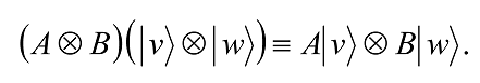
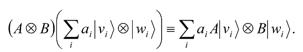
Suppose |vâ© and |wâ© are vectors in V and W, and A and B are linear operators on V and W, respectively. Then we define a linear operator A⊗B on V⊗W by the equation
The definition of A⊗B is then extended to all elements of V⊗W in the natural way to ensure linearity of A⊗B, that is,
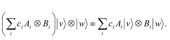
One can show thatA⊗B so defined is a well-defined linear operator on V⊗W. This notion of the tensor product of two operators extends in the obvious way to the case where A: V→V’ and B: W→W’ map between different vector spaces. Indeed, an arbitrary linear operator C mapping V⊗W to V’⊗W’ can be represented as a linear combination of tensor products of operators mapping V to V’ and W to W’,
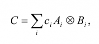
where by definition
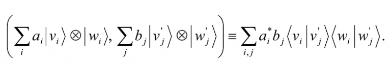
The inner products on the spaces V and W can be used to define a natural inner product on V⊗W.
Define
42 A† ≡ (AT)* ≡ (A*)T is the Hermitian conjugate or adjoint of matrix A. An operator A whose adjoint is also A is known as a Hermitian or self-adjoint operator.
It can be shown that the function so defined is a well-defined inner product. From this inner product, the inner product space V⊗W inherits other familiar structures, such as notions of adjoint, unitarity43, normality, and Hermiticity.
A.5.7 Congruence Modulo
The expression a ≡ b mod m is read as “a is congruent to b modulo m.” Let m ≠ 0 be an integer. We say two integers a and b are congruent modulo m if there is an integer k such that a-b = km, i.e., (a-b)/m is an integer. A familiar example of this form of arithmetic is the clock. Clocks use modular arithmetic with modulus 12 for displaying hours (as there are 12 hours on the clock face), and modulus 60 for displaying minutes (as there are 60 minutes in an hour).
Note that here the symbol ‘≡’ is not equality but congruence44, and the ‘mod m’ signifies the number by which b must be divided to get k and the remainder a. The remainders can be 0, 1, 2,… , m-1. Integer numbers thus get classified into m residue classes (also called congruence classes) labelled, respectively, by the remainders 0, 1, 2,… , m-1. For m = 2, the classes are:
[0] = {…, 4, 2, 0, 2, 4, …}
[1] = {…, 3, 1, 1, 3, 5, …}
Modulo arithmetic is done, digit by digit, on binary numbers. Each digit is considered independent of its neighbors. Numbers are not carried or borrowed.
The following addition rules for adding two binary numbers are obvious:
0 + 0 ≡ 0 (mod 2), 0 + 1 ≡ 1 (mod 2), 1 + 0 ≡ 1 (mod 2), 1 + 1 ≡ 0 (mod 2).
In modulo 2 arithmetic, the addition operation is the XOR (or Cnot) operation. It is carried out on the corresponding binary digits of each operand according to the following rule:

The above rules may also be interpreted as “the sum of even numbers is even”, “the sum of an even number and an odd number is odd”, “the sum of an odd number and an even number is odd”, and “the sum of two odd numbers is even”, respectively, in modulo 2 arithmetic.
The following multiplication rules for multiplying two binary numbers are also obvious:
0 x 0 ≡ 0 (mod 2), 0 x 1 ≡ 0 (mod 2), 1 x 0 ≡ 0 (mod 2), 1 x 1 ≡ 1 (mod 2).
In modulo 2 arithmetic, the multiplication operation is the Boolean AND operation45:
0 ^ 0 = 0, 0 ^ 1 = 0, 1 ^ 0 = 0, 1 ^ 1 = 1.
Thus, we have a system with addition and multiplication, but in which the only numbers that can exist are 0 and 1.
43 A n×n matrix U is unitary if U†U = UU† = I, where I is the unit matrix. This condition means that U is unitary if and only if it has an inverse which is equal to its conjugate transpose U†.
44 Coinciding exactly when the remainders are compared.
45 The symbol ∧ represents the word “AND”.
Fourier series and analysis
The weirdness of quantum mechanics is that a quantum object shows both particle-like and wave-like behavior. An understanding of waves and Fourier analysis is therefore central to quantum computing.
In physics, all systems which oscillate harmonically are quantized in terms of their energy, whether these systems are material oscillators, sound waves, or electromagnetic waves. Since we see diverse systems interacting with each other, it follows that the quantization of any one type of harmonic oscillator will require a similar quantization of all other types. Reflection, refraction, interference, and diffraction are characteristic behaviors of all types of wave46.
Interference is the test for wave motion. In quantum mechanics, of primary interest are probability waves that give the probability amplitude of finding a particle at a given place—the so-called “matter waves”. Their frequency is proportional to the energy and their wave number is proportional to the momentum of the particle. Complex algebra amazingly allows us to calculate the striking interference effects seen in quantum phenomena. Fourier analysis allows us to estimate the period from a discrete set of values sampled at a fixed rate.
The finite, or discrete, Fourier transform of a complex vector y with n elements yj is another complex vector Y, also with n elements Yk47:
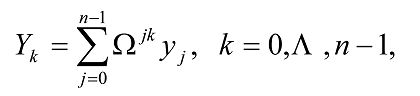
where Ω is a complex n-th root of unity given by
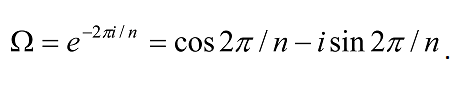
In matrix notation, the above Fourier transform can be expressed as
Y= Fy,
where the elements of the matrix F are given by
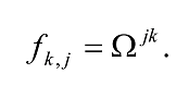
It can be shown that
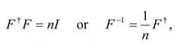
which then allows us to invert the Fourier transform:
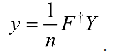
Hence
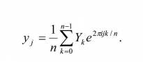
It is obvious that F√n is unitary. A direct application of the Fourier transform
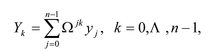
requires n multiplications and n additions for each of the n components of Y for a total of 2n2 floating-point operations in addition to the operations required to generate the powers of Ω . Smart calculation strategies, generally known as fast-Fourier transform (FFT) algorithms are able to do the calculations in
O(n log2 n) floating-point operations instead of in O(n2) operations 48. The importance of Fourier analysis in quantum computing became evident once it was realized that quantum computers could perform a type of Fourier transform much faster than classical computers. This enabled many important quantum algorithms to be developed.
46 See: Wave Behavior, http://www.aktsunami.com/lessons/9-12/unit6/9-12_3WaveBehavior.pdf,
http://hyperphysics.phy-astr.gsu.edu/hbase/sound/p2032.html for an elementary school-level recap on waves; and
VanCleave (2006). VanCleave, J. P. Janice VanCleave’s Energy for Every Kid. Hoboken, Wiley & Sons, N.J. 2006.
47 See, e.g., MATLAB, Chapter 8, Fourier Analysis, http://www.mathworks.com/moler/fourier.pdf
48 See, e.g., Press, W. H., Teukolsky, S. A., Vetterling, W. T., and Flannery, B. P. Numerical Recipes in C. Cambri.ge Press, Cambridge, Second Edition, 2002. https://www2.units.it/ipl/students_area/imm2/files/Numerical_Recipes.pdf