It now appears that quantum computers are poised to enter the world of computing and establish its dominance, especially, in the cloud. Turing machines (classical computers) tied to the laws of classical physics will not vanish from our lives but begin to play a subordinate role to quantum computers tied to the enigmatic laws of quantum physics that deal with such non-intuitive phenomena as superposition, entanglement, collapse of the wave function, and teleportation, all occurring in Hilbert space. The aim of this 3-part paper is to introduce the readers to a core set of quantum algorithms based on the postulates of quantum mechanics, and reveal the amazing power of quantum computing.
Key words: Quantum mechanics, quantum computing, quantum algorithms.
In Part 1 we introduce certain fundamental differences between classical and quantum physics. They lead to vastly different means of computing. Indeed, the very idea of the state of a system in quantum mechanics is conceptually different from its classical counterpart. In each, states are represented by different mathematical objects and have a different logical structure. In classical physics, the state of a system describes everything that is required to predict the future of that system. It is not so for a quantum system. The state of a quantum system is neither completely measurable nor completely predictable. We conclude this part by describing a set of quantum operators and their essential features that enable quantum computing by exploiting such exotic quantum features as superposition, entanglement, and collapse of the wave function. Part I comprises Sections 1-8 of the paper. In Part II comprising Sections 9-11, we will describe a range of quantum algorithms to display the tremendous computing power waiting to be unleashed via controlled superposition and entanglement of quantum states, and collapse of the wave function. In Part III we speculate on the quantum measurement conundrum and comment on the future of quantum computing.
Caution: Leave your intuition and common sense behind. Ask not what quantum computing can do for you, ask what you can do for quantum computing. You are about to enter a world where disbelief reigns.
Scientific discoveries are based on conjectures and refutations2. It will always remain so. As of now, quantum theory contains our most fundamental knowledge of the physical world. It is a very different description of Nature from classical physics described by Galileo, Newton, Maxwell, and Einstein. A law of Nature states what is possible within certain inviolable boundaries.
I expect readers, not trained in quantum mechanics, to be confused, especially if they have heard such weird stories as a cat being simultaneously dead and alive, the phenomenon of teleportation, a photon or an electron concurrently traveling along two paths, and so on. Rest assured even established researchers in quantum mechanics struggle to develop an intuition about the subject. Einstein once remarked, Quantum Mechanics: Real Black Magic Calculus. And Niels Bohr said, “If quantum mechanics hasn’t profoundly shocked you, you haven’t understood it yet.”
It pays to view quantum mechanics as a mathematical framework for constructing physical theories and concentrate on grasping the rules of the game. Explore the subject as if trying to understand an alien world. Patience and diligence will be handsomely rewarded because what will be revealed is the finest set of scientific conjectures created by the human mind to date.
As a deeper understanding of Nature via physics evolved so did the mathematical complexity of the Laws of Nature that describe it in the sense that mental visualization by means of interpreting those abstractions has become increasingly difficult. Later laws have generally required more sophisticated (abstruse) mathematics, which has placed a heavy burden on people trying to understand Nature. Indeed, “it is impossible to explain honestly the beauties of the laws of nature in a way that people can feel, without their having some deep understanding of mathematics.”4. We communicate through language and emotion. Benjamin Lee Whorf (1897– 1941) said, “Language shapes the way we think, and determines what we can think about.” And Ludwig Wittgenstein (1889 –1951) said, “The limits of my language mean the limits of my world.” It is more so with mathematics because it is both a language and a tool for reasoning. It also requires extreme mental discipline and meticulous training. It is amazing that as mathematics continued to enrich itself through new explorations (e.g., calculus, fractal geometry, etc.) it also enabled physicists expand their understanding of Nature.
So, keep a standard text book on mathematics nearby for ready reference (e.g., Kreyszig5, Chapters 7-12). A good understanding of linear algebra and Fourier analysis is necessary. Further, abandon common sense like the plague. Just stick to the postulates of quantum mechanics and their underlying mathematics. Do not add or subtract unless you want to rewrite quantum mechanics.
The remarkable, 1936 paper by Alan Turing6 provides a mathematical description of all classical computers—from Charles Babbage’s analytical engine7 to the supercomputers of today—known as the Universal Turing Machine (UTM). It was conceived before there were any real computers. The UTM perfectly mimics an unintelligent person, who tirelessly and with absolute concentration, performs calculations as instructed, in a step-by-step manner, i.e., according to a given algorithm. This Turing Person has at its disposal unlimited time, paper, pencil, and energy. Note that the UTM does only those tasks that a human might do in executing an algorithm without the help of insight. There is a strong belief, so far unrefuted, among computer scientists that what is human-computable is machine-computable. This is the famous Church-Turing Thesis: “The class of functions computable by a Turing machine corresponds exactly to the class of functions which we would naturally regard as being computable by an algorithm.”8 It is also a statement about the limitations of the human mind.
Through mathematical abstraction, Turing captured the essence of algorithmic processes and ushered in the modern computer revolution. He thus revealed a very mechanistic aspect of reality that there may be nothing more to mind, brain, or the physical world than ceaseless computation. Max Tegmark expresses this idea even more explicitly: “Our reality isn’t just described by mathematics – it is mathematics … Not just aspects of it, but all of it, including you.” In other words, “our external physical reality is a mathematical structure”10. One might thus conclude the Universe is a computer and hence the Laws of Nature must be computable. While a physical UTM does use quantum processes, its actual construction, by design, suppresses all quantum effects.
[2] Popper (1963).
[3] As quoted in Vizzotto, Altenkirch, & Sabry (2005).
[4] Feynman (1965), pp. 33-34.
[5] Kreyszig (2011).
[6] Turing (1936).
[7] Charles Babbage (1791-1871) was Lucasian Professor of mathematics at Cambridge from 1828 to 1839. He was the first to describe a programmable computer.
[8] Nielsen & Chuang (2000), p. 125.
[9] Aaronson (2013).
[10] Tegmark (2014), p. 254.
The very concept of the state of a system in quantum mechanics is different from its classical counterpart. In each, states are represented by different mathematical objects and have a different logical structure. In classical physics, the state of a system describes everything that is required to predict the future of that system. It is not so for a quantum system. The state of a quantum system is neither completely measurable nor completely predictable. Consequently, each system is interpreted differently. Each perspective demands a different mindset through which ideas, concepts, and interpretations flow. Even though certain formal terms, e.g., space, time, momentum, measurement, superposition, etc. are used in both systems, their mathematical underpinnings and mental interpretation are different. From either perspective, the other looks weird and apparently incompatible.
For example, in classical physics, Einstein’s general relativity describes gravity as the warping of space-time in the presence of mass, but to know what happens inside a massive black hole or what happened at the big bang requires a quantum mechanical explanation. The extremely weak gravitational waves predicted by Einstein were detected on 14 September 201511 and the Nobel Prize for physics (2017) promptly awarded to Rainer Weiss, Barry C. Barish, and Kip S. Thorne “for decisive contributions to the LIGO detector and the observation of gravitational waves”12. It is likely that quantum entanglement (explained below) may provide an answer.13 For other differences pertinent to the present paper see Sections 3.1, 3.2, and 4.
The deeper we explore Nature, its laws become “more and more unreasonable and more and more intuitively far from obvious.”14 So it has been from Newton’s laws of motion to Maxwell’s equations of electromagnetism to Einstein’s general theory of relativity to the postulates of quantum mechanics. The last are so baffling that Richard Feynman said:
I am going to tell you what nature behaves like. If you will simply admit that maybe she does behave like this, you will find her a delightful, entrancing thing. Do not keep saying to yourself, if you can possibly avoid it, ‘But how can it be like that?’ because you will get ‘down the drain’, into a blind alley from which nobody has yet escaped. Nobody knows how it can be like that.15
Here are a few examples of the strangeness of quantum mechanics, the crown jewel of physics.
Classical physics presupposes that exact simultaneous values can be assigned to all physical quantities; quantum mechanics shows there are exceptions, e.g., the position and momentum of a particle. In such cases, the more precisely one quantity is measured, the less precisely can the other be measured. (See Heisenberg’s uncertainty principle in Section 4.4.)
Classical physics assumes that it is possible to measure the state of a system so delicately that it does not noticeably interfere with the system. In the quantum world it is simply impossible. Further, we intuitively assume that identical conditions always produce identical results. This too fails in quantum mechanics; it produces statistical results. When combined with the previous paragraph, it means that we cannot define the trajectory of a particle in quantum mechanics.
Unlike classical physics, in quantum mechanics there is no gradual transfer of energy from radiation field to matter. Planck’s assumption that energy transfer is a discontinuous process and is quantized has been amply confirmed by experiments.16
In Section 4.4, we present other quite crucial differences between classical and quantum physics. Taken together, it makes one wonder if every quantum bit (qubit) in a quantum computer is so different from a classical bit, how does a quantum computer work. The answer lies in making very clever use of superposition and entanglement of quantum states and in collapsing them.
| See Fig. 3.1.17 What did you see? Likely, a young woman (if you had gazed up; call it state |0 of the picture in quantum mechanical notation) or an old woman (if you had gazed down; call it state |1 of the picture)! You did not see some weird superposition (or summation) of the two. Although both coexist in the picture, each observer will see, at random, one or the other at a given time, independent of what others see then or at another time. It is in this metaphorical sense a quantum object is said to be in a state of superposition. Without any prior knowledge of the picture a viewer would randomly gaze up or down and accordingly see a young or an old woman. From a group of viewers, each of whom was shown an identical copy of this picture, you would get a statistical sample of the fraction of people who tend to look up or look down. Quantum systems when measured produce statistical results. Just as you did not see Fig. 3.1 as the sum of a young and an old woman, in quantum systems you can never see the system in its superposed state. You can only see one of its eigenstates, randomly chosen by Nature, and collect statistics. Where Fig. 3.1 differs from a quantum system is that no amount of observation will change the picture nor its effect on an observer. The state of the picture (a classical object) is immune to observation. A quantum object is not. A quantum object, when first observed, freezes (collapses) into the state it has revealed to the observer, and subsequent observations will reveal only the frozen state. Of course, there are means that can put the object into its original state (only if the original state is known) or some other state. |  |
The response of two entangled quantum objects (metaphorically, as paired dance partners), to any change of state in one (e.g., due to its being observed) is an instant reactive change in the other independent of any distance separating them. The action implies perfect coordination without the benefit of anticipation. Perfect coordination in the classical world is possible only with preplanning, e.g., by following an agreed upon schedule of events.
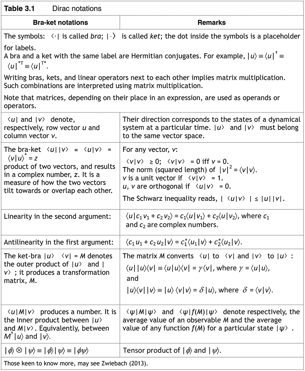
Notations and the meanings we attach to them encode knowledge. In Table 3.1, we provide a few symbols and their frequently used combinations in quantum mechanics for easy reference. Familiarization requires only elementary pattern recognition skills. The notations were invented by Paul Dirac (1902-1984)18 in 1939 as a kind of dress code for quantum physicists to show off (just kidding!). He is one of the founders of quantum mechanics, and while founding, predicted the existence of antimatter, and won the Nobel Prize in Physics for it in 1933, at age 31.
In quantum computing, one talks about Hilbert space only to impress people. It is really about formatting of matrices—creating larger matrices by patching together smaller ones (the tensor product). It turns out that in the finite dimensional complex vector spaces that come up in quantum computing and quantum information, the Hilbert space is exactly the same thing as an inner product space. Also, beware that what appears as a variable in classical mechanics may appear as an operator in quantum mechanics. In natural languages, nouns becoming verbs and vice-versa are not uncommon. In classical physics, e.g., momentum is a variable but an operator in quantum physics.â©
The simplest object that allows a state change is one with two states. We conventionally and arbitrarily label one as state 0 and the other as state 1 and provide rules for state change. While the classical binary bit at any given time can be either in state 0 or state 1, its counterpart the quantum bit, christened qubit by Ben Schumacher,19 can be and usually is in some superposition of the two quantum states |0â© and|1â©. The general state representation of a qubit is the unit vector α|0â© + |1â© where and are complex numbers, constrained by |α|2 + |β|2 = 1. Unless |α| or |β| = 1, the qubit is in a state of superposition.
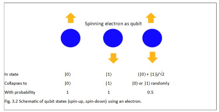
This qubit when observed (i.e., its state measured), will be seen in either state |0â© or state |1â© according to a statistical rule, i.e., given a very large number of identical copies of the qubit and each copy measured, the qubit will collapse to state |0â© with probability |α|2 and to |1 with probability |β|2. This insightful, probabilistic aspect of Nature was uncovered by Max Born for which he received the 1954 Nobel Prize in Physics20. A quantum system, when appropriately observed or measured, randomly collapses to only one of its eigenstates |0â© or |1â© according to Postulate 3 in Section 4.1.
Two or more qubits can be entangled, and if handled with care, can be separated very far apart. Entanglement is a joint characteristic of two or more quantum particles. All interesting quantum algorithms make clever use of entanglement. As you gain experience with entanglement, you will see it as an enormous computing resource unknown in classical physics. As an aside, note that a qubit in the superposed state α|0â© + β|1â© may be viewed as being in a state of self-entanglement, because when α changes so does β instantly.
In a physical computer, qubits are physical objects (e.g., photons, electrons), which unless extremely well shielded, tend to randomly entangle with their environment. This decoheres their state of superposition and hence the information they encode. Thus, long computations are difficult to sustain. This is a hardware issue, but clever error correcting algorithms encoded in software for certain situations exist21. For an excellent tutorial on decoherence, see Marquardt and Püttmann.22
A quantum system is described by its state vector, |Ψâ©. Its mathematical description and evolution is enshrined in the enigmatic postulates of quantum mechanics. Any system that fulfills the postulates is quantum mechanical. The postulates encompass all the observed weirdness of quantum systems described in Sections 3.1 and 3.2 and some more. The postulates neither tell us how a quantum system knows it is being observed nor the mechanism related to the collapse of | Ψâ© when it is observed.
Note: The superscripts *, T, and † ( *T = T*) attached to various symbols, respectively, denote complex conjugate, transpose, and Hermitian conjugate (or adjoint) operations on the symbol.
[11] Abbott, et al (2016).
[12] RSAS (2017); Resnick (2017).
[13] Bose, et al (2017).
[14] Feynman (1965), Chapter 6.
[15] Feynman (1965), Chapter 6.
[16] This even includes data collected on the background radiation at the edge of the universe (remnants of the Big Bang) by the COBE satellite in 1990. The data fits perfectly Planck’s black-body radiation law. See, e.g., RSAS (2006).
[17] Picture credit: William Ely Hill (1887–1962), My wife and my mother-in-law, https://en.wikipedia.org/wiki/My_Wife_and_My_Mother-in-Law (in public domain)
[18] Dirac (1939). See also: Gidney (2016).
[19] Schumacher (1995). See also: Preskill (2015).
[20] Born (1954).
[21] Shor (1995).
[22] Marquardt & Püttmann (2008).
The four postulates of quantum mechanics have no resemblance to the postulates of Newtonian mechanics. The quantum postulates are, as given in Nielsen and Chuang23:
Postulate 1: Associated to any isolated physical system is a complex vector space with inner product (that is, a Hilbert space) known as the state space of the system. The system is completely described by its state vector, which is a unit vector in the system’s state space.
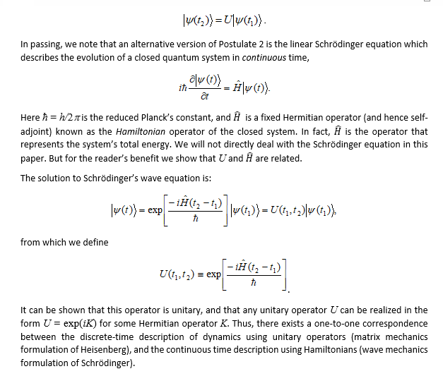
Postulate 2: The evolution of a closed quantum system is described by a unitary transformation. That is, the state |Ψ(t1)â© of the system at time t1 is related to the state |Ψ(t2)â© of the system at time t1 by a unitary operator U which depends only on the times t1 and t2, i.e.,
Postulate 3: Quantum measurements are described by a collection {Mm} of measurement operators. These are operators, which act on the state space of the system being measured. The index m refers to the measurement outcomes that may occur in the experiment. If the state of the quantum system is |Ψâ© just before the measurement, then the probability that result m occurs is given by
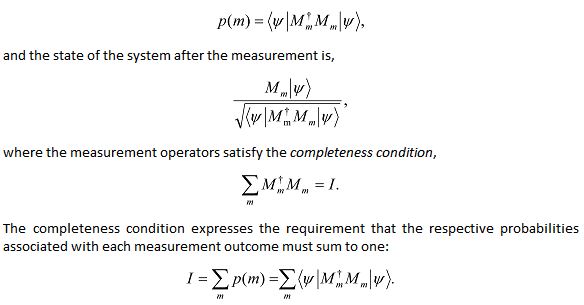
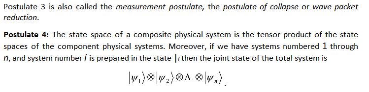
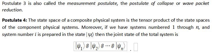
The four postulates are independent of one another. Postulates 1 and 4 describe the mathematical state space in which quantum mechanical systems live and act. It asserts that a quantum system is completely described by its state vector, |Ψâ© , which is a unit vector in the system’s state space. Postulate 2 describes the evolution of a quantum system as described by its state vector |Ψâ© . Postulate 3 describes the post-measurement, collapsed state of |Ψâ©.
The evolution of |Ψâ© under Postulate 2 is completely deterministic, continuous, and smooth. Its value, even using proxies, cannot be determined by any classical measurement system. Its evolution is governed by the Schrödinger wave equation, which provides the rate at which |Ψâ© changes. In fact, the heart of quantum theory is Postulate 2 once we know how to interpret |Ψâ© according to Postulate 3. There are no probabilities involved in Postulate 2.
Postulate 3 asserts that any legitimate classical measurement on |Ψâ©, in general, will yield only partial, non-deterministic information about the system’s state immediately prior to the measurement. The very first measurement on a system will irreversibly “collapse” |Ψâ© and do so in a probabilistic manner. Measurement overrides Postulate 2. It is not possible to know |Ψâ© of an unknown quantum system completely by making multiple measurements on the same system or even on multiple copies of the system. Since all the probabilities associated with quantum mechanics are contained in Postulate 3, a knowledge of probability is essential to analyze measured data. Measurement is an irreversible process. Once a measurement is made, the previous history of |Ψâ© is lost. Postulates 2 and 3 appear conflicting. F. Laloë articulates the conflict.
Obviously, having two different postulates for the evolution of the same mathematical object is unusual in physics; the notion was a complete novelty when it was introduced, and still remains unique in physics, as well as the source of difficulties. Why are two separate postulates necessary? Where exactly does the range of application of the first stop in favor of the second? More precisely, among all the interactions – or perturbations – that a physical system can undergo, which ones should be considered as normal (Schrödinger evolution), which ones as a measurement (wave packet reduction)? Logically, we are faced with a problem that did not exist before [in classical physics], when nobody thought that measurements should be treated as special processes in physics.24
Roger Penrose25 too describes the weirdness of the postulates. In his view, in quantum mechanics there exists two completely different postulates those describe the evolution of |Ψâ©. Postulate 2 is totally deterministic, whereas Postulate 3 is probabilistic; Postulate 2 maintains quantum complex superposition, but Postulate 3 grossly violates it; Postulate 2 acts in a continuous way, Postulate 3 is blatantly discontinuous. There is nothing in quantum mechanics that even implies that one can ‘deduce’ Postulate 3 as a complicated instance of Postulate 2. Postulate 3 is simply a different procedure and it contains all the non-determinism found in the theory. It replaces superposition with a definite state. Both postulates are needed for all the marvelous agreements that quantum theory has consistently provided with observational facts. What is missing is a clear rule that would tell us when the probabilistic Postulate 3 should be invoked, in place of Postulate 2.
[23] Nielsen & Chuang (2000). pp. 80-94.
[24] Laloë (2001).
[25] Penrose (1989), p. 323.
The state vector |Ψâ© is an abstract mathematical entity; its origin and any underlying sub-quantum structure it might have is unknown. The processes that comprise measurement too are unknown. In our experience, certain physical interactions are recognizably ‘measurements’, but there are unknown others which are not. Their incognito presence makes the building of robust quantum computers difficult because they can surreptitiously destroy the quantum superposition of the state vector |Ψâ©. There is deeply mysterious, unexplained physics.
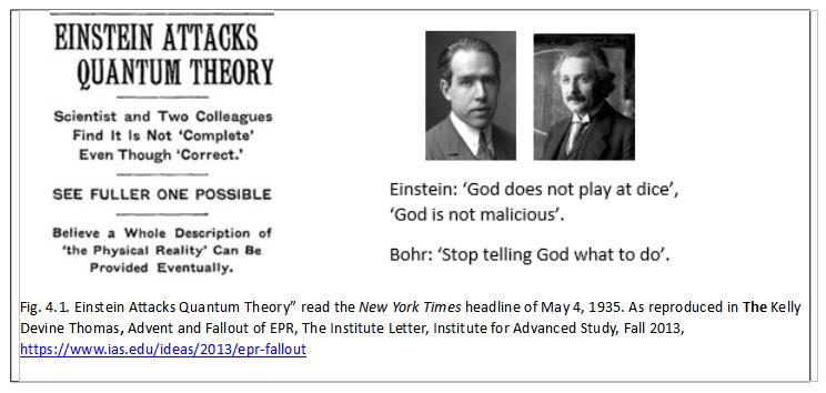
Entanglement, disdainfully viewed by Einstein, Podolsky, and Rosen (EPR) as spooky action at a distance26, comes from postulates 1, 2 and 4. It implies that information can travel instantly from place to place unmindful of distance rather than at a finite speed capped by the speed of light as Einstein had postulated, unless there exist pre-programable “hidden variables” which control the system. Quantum mechanics was therefore incomplete in their view. This is the famous EPR paradox. Bohr promptly rebutted and promoted his complementarity theory27. The spat between Einstein and Bohr drew a lot of media attention too (see Fig. 4.1).
In 1964, John Stewart Bell brilliantly ruled out the necessity of hidden variables in explaining entanglement. The result is famously known as Bell’s theorem.28 Entanglement is a physically observable phenomenon; entangled particles are now routinely produced in experiments.
In 1982, Aspect, et al29 provided experimental evidence of entanglement. In February 2017, even more stringent experimental evidence of entanglement was provided by Handsteiner, J., et al30. Thus, when two or more particles are entangled, a measurement on any one particle or a combined measurement on a subgroup of particles will cause a ‘collapse’ to occur instantly on the remaining particles no matter where they are in the Universe. A group of entangled particles thus have a distributed existence yet function as a single unit.
The existence of entangled states in a composite system remains an enigma. The word ‘entanglement’ (in German, ‘Verschrankung’) was introduced by Schrödinger (among the first people to realize its strangeness) in the early days of quantum mechanics. To get an inkling of entanglement, consider a two-qubit system with the qubits labeled 1 and 2 with respective state vectors |Ψ1â© = α1|0â© + β1|1â© and |Ψ2â© = α2|0â© + β2|1â© . Therefore, any state of the form |Ψ1â© ⊗ |Ψ2â© ≡ |Ψ1Ψ2â© in this composite two-qubit system can be written as
|Ψ1Ψ2â© = α1α2|00â© +α1β2 |01â© +α2β1 |10â© + β1β2 |11â© ,
where the coefficient of each of the four basis vectors — |00â©, |01â©, |10â©, |11â© — is interpreted as a probability amplitude. For example, |α1β2|2 gives the probability of finding qubit 1 in state |0â© and qubit 2 in state |1â© if the two-qubit system is measured. In this two-qubit system, we notice something unusual. For example, the so-called Bell state
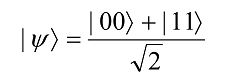
has the remarkable property that there is no single qubit states |aâ© and |bâ© such that |Ψâ© = |aâ© ⊗ |bâ© . A state of a composite system which cannot be written as a product of states (factorized) of its component systems is called an entangled state. Entanglement is a form of quantum superposition.
Factorizable states can be explained as follows. Let Alice and Bob each possess a qubit. Suppose, now, that Alice and Bob prepare their qubits independently, where both operations may depend on the output of a classical random number generator, e.g., a dice. Therefore, the source of the correlations is a classical random number generator. The two-qubit states which Alice and Bob can prepare in this way using their respective dice are called classically correlated or separable. All other two-qubit states are called entangled. Separable states occur because the dice are not related to each other. If the dice were related, (e.g., if one dice showed 2 the other would invariably show 5, etc.) the result would have been entangled states. Clearly, related dice function as a unit and can only acquire a group state.
Since an entangled state cannot be factorized, it is impossible to specify a pure state of its constituent components; we can only specify a group state. Interestingly, this group state is a pure state in the Hilbert space! In other words, we have knowledge of the correlation between measurement outcomes on qubits 1 and 2 but we cannot, in principle, identify a pure state with each of the qubits 1 and 2 individually. Entanglement is a fundamental difference between classical and quantum physics.
Abstract mathematical statements, if they are to describe the world to a human mind, need an isomorphic interpretation that establishes a correspondence between mathematical symbols and the rules by which those symbols are aggregated on the one hand and entities and mental concepts about our Universe on the other. The correspondences we discover may be many. When that happens, we seek a more unified view of our Universe by drawing analogies among the correspondences. In this Section we provide three well-known interpretations of quantum mechanics. The conceptual diversity of these interpretations is remarkable. In Part III, a sub-quantum level view of the quantum world is presented.
[26] Einstein, Podolsky & Rosen (1935).
[27] Bohr (1935).
[28] Bell (1964).
[29] Aspect, Dalibart & Roger (1982). See also Aspect (1991).
[30] Handsteiner, et al (2017). See also: Hensen, et al (2015); and Merali (2015).
The Copenhagen interpretation, named after the city in Denmark where Bohr lived and worked, was provided by Niels Bohr and Werner Heisenberg around 1927. It is the most cited Interpretation. It extends the probabilistic interpretation of the wave function proposed by Max Born.31 As Jammer notes:
The Copenhagen view is not a single, clear-cut, unambiguously defined set of ideas but rather a common denominator for a variety of related viewpoints.32
The interpretations’ interesting features include: the position of a particle is essentially meaningless; a measurement causes an instantaneous collapse of the wave function and the collapsed state is randomly picked to be one of the many possibilities allowed for by the system’s state vector; the fundamental objects handled by the equations of quantum mechanics are not actual particles that have an extrinsic reality but “probability waves” that merely have the capability of becoming “real” when an observer makes a measurement. Even then it does not explain entanglement; this observed “nonlocality” is a mathematical consequence of quantum theory33. In Bohr’s view,
there is no quantum world. There is only abstract quantum physical description. It is wrong to think that the task of physics is to find out how nature is. Physics [only] concerns what we can say about nature34(p153) .
This view is contrary to Einstein’s who believed that the job of physical theories is to ‘approximate as closely as possible to the truth of physical reality.35’ David Merman once dubbed the Copenhagen interpretation as the ‘shut up and calculate’ interpretation.36
Everett’s many world interpretation
Hugh Everett III, in his 1956 doctoral dissertation37 (journal version38), proposed his “relative state interpretation”, now generally known as the many world interpretation (the name was coined by Bryce DeWitt in the late 1960s). This interpretation is perhaps the most bizarre and yet perhaps the simplest because it circumvents the measurement conundrum. Everett posits that when a quantum system is faced with a choice as in a measurement, the entire Universe splits into a number of universes equal to the number of collapse-choices available. When a universe splits, observers in it also split. Thus, there will be parallel copies of observers in parallel universes, each of whom will see the specific outcome that appears in his respective split universe39. Variants of the many-world interpretation are the multiverse interpretation, the many-histories interpretation, and the many-minds interpretation.
Physicists, including Bohr, at the time ridiculed Everett’s interpretation (he got his PhD alright and the work was published). It was said that “Bohr gave him the brush-off when Everett visited him in Copenhagen.40” He was so discouraged by the ridicule that he left physics, became a defense analyst, then a private contractor to the U.S. defense industry which made him a multimillionaire41. “Everett advised high-level officials in the Eisenhower and Kennedy administrations on the best methods for selecting hydrogen bomb targets and structuring the nuclear triad of bombers, submarines and missiles for optimal punch in a nuclear strike.”42 Everett is also renowned for his generalized Lagrange multiplier method. After Everett’s death, his interpretation has gained widespread respect of physicists, especially of David Deutsch who believes:
The quantum theory of parallel universes is not the problem, it is the solution. It is not some troublesome, optional interpretation emerging from arcane theoretical considerations. It is the explanation, the only one that is tenable, of a remarkable and counter-intuitive reality.44
In Bohm’s interpretation45, which appeared in 1952 predating Everett’s, the whole universe is entangled, and one cannot isolate one part of the universe from the other. In Bohm’s view, the interaction between entangled particles is not mediated by any conventional field known to physics (such as the electromagnetic field), but by an all-pervasive field that is instantaneous. He showed that the non-local interactions can be described in terms of a very special anti-relativistic quantum information field (pilot-wave) that does not diminish with distance and that binds the whole universe together. This field is not physically measurable but manifests itself in terms of non-local correlations. The idea is not only interesting but entirely derivable from the Schrödinger equation. Consequently, in Bohm’s interpretation, e.g., the electron is a particle with well-defined position and momentum at any instant. However, the path an electron follows is guided by the interaction of its own pilot wave with the pilot waves of other entities in the universe. A major supporter of Bohm’s interpretation was John Bell.
[31] Born (1926a); Born (1926b).
[32] Jammer (1974), p. 87. Quotation as reproduced in Al-Kahlili (2003), p. 134.
[33] Seife (2005)
[34] Al-Kahlili (2003).
[35] Al-Kahlili (2003), p. 153.
[36] Mermin (2004
[37] Everett (1957a).
[38] Everett (1957b).
[39] Byrne (2007).
[40] Al-Kahlili (2003).
[41]Al-Kahlili (2003).
[42] Byrne (2007).
[43] Everett (1963).
[44] Deutsch (1997), p. 51.
[45] Bohm & Hiley (1993), Chapter 3. The original paper is: Bohm (1952).
A desire to understand Nature is an attempt to minimise an information gap – the information we try to prise from Nature and Nature’s ability to withhold by making us run around in circles.
Physics gives rise to observer-participancy; observer-participancy gives rise to information; and information gives rise to physics46. – John Wheeler
What we call the laws of physics is the information we extract from Nature, compact and package within a falsifiable conjecture which we have so far failed to refute. We are forced to conjecture (or hypothesize) and endlessly refine, discard, and amend our conjectures by strenuously trying to refute them because Nature appears determined to be secretive.47 Since our present best understanding of the Universe is enshrined in quantum mechanics, it appears natural to agree with David Deutsch: “Our best theories are not only truer than common sense, they make more sense than common sense.”48 The consequences of the postulates are strikingly non-intuitive. Here are some examples.
Heisenberg’s uncertainty principle. In 1927, Heisenberg showed that both the position and the velocity of a quantum object cannot be simultaneously measured exactly, even in theory. Further, this restriction cannot be overcome by refining the measuring apparatus or techniques. The classical concept of exact position and exact velocity being measured simultaneously is barred in quantum mechanics. It is a limit imposed by Nature as we penetrate into the subatomic world. Heisenberg originally stated his uncertainty principle, based on how waves behave in classical physics, as follows: If q is the error in the measurement of any coordinate and p is the error in its canonically conjugate momentum, then
Δp Δq≥ h/2.
The modern and correct interpretation of Heisenberg’s uncertainty principle is in terms of the standard deviation and the commutator operator rather than the earlier misconceived notion that the uncertainty principle is about measuring a quantity C to some ‘accuracy’ Δ(C) which then causes the value of D to be ‘disturbed’ by an amount Δ(D) in such a way that some sort of inequality is satisfied. Mathematically, given a large number of identical quantum systems each in state |Ψâ©, suppose we measure C on some of those systems, and D in others, where C and D are represented by two observables (represented by operators), then the standard deviation Δ(C) of the C results times the standard deviation Δ(D) of the results for D will satisfy the inequality49
Δ(C)Δ(D)≥ |â¨Ψ|[C,D]|Ψâ©| / 2
This is the content of Heisenberg’s Uncertainty Principle50. It imposes a fundamental limit on the sharpness of the dynamics (courtesy the Planck’s constant) by preventing us from even talking about initial conditions since we cannot know the exact position and velocity of a particle simultaneously. Hence, it prevents us from even talking about trajectories. Thus, indeterminism is built into the very structure of matter where certain pairs of variables (such as position and momentum) cannot even exist simultaneously with perfectly defined values.
In the most extreme case, absolute precision of one variable in a pair would entail absolute imprecision regarding the other. This is in sharp contrast to classical physics where “if we know the present exactly, we can calculate the future”. The Uncertainty Principle says the opposite: it is not the conclusion that is wrong but the premise. One cannot calculate the precise future motion of a particle, but only a range of possibilities for its future motion. (However, the probabilities of each motion, and the distribution of many particles following these motions, can be calculated exactly from Schrödinger’s wave equation.) It is thus not possible to make a complete mental picture of events in the quantum world. Heisenberg concluded:
The mathematically formulated laws of quantum theory show clearly that our ordinary intuitive concepts cannot be unambiguously applied to the smallest particles. All the words or concepts we use to describe ordinary physical objects, such as position, velocity, color, size, and so on, become indefinite and problematic if we try to use them of elementary particles.51
At the mental level, we feel we understand the large-scale world only when we have developed a mental picture of it. Newtonian mechanics pandered to that mental level by dealing with measurable and observable quantities such as position, velocity, etc. Quantum events cannot be pictured in our mind, and therefore it leaves us with the queasy feeling that it is unreal, further strengthened by the fact that quantum mechanics deals with not real numbers but complex numbers.
Complementarity. In classical physics, particles and waves behave distinctly differently. In quantum mechanics, an object may behave in either way! In fact, Bohr’s complementarity principle (or wave-particle duality) states that a quantum object can behave either as a particle or as a wave, but never as both simultaneously.52 At the quantum level, both particle and wave aspects of reality are equally significant. However, the wave character is not a physical vibration but rather a wavelike function that encodes information about where a quantum entity will be found once it is detected.
Position is a precisely locatable particle property; waves have no precise location, but they have precise momentum. Heisenberg’s uncertainty principle seems to say that the observer can choose which aspect of Nature he wants to observe and with what precision.
About complementarity, John Wheeler remarked,
Bohr’s principle of complementarity is the most revolutionary scientific concept of this century and the heart of his fifty-year search for the full significance of the quantum idea.53
[46] Wheeler (1989), pp. 313-314.
[47] Popper (1963).
[48] Deutsch (2009).
[49] For a proof, see Nielsen & Chuang (2000), p. 89.
[50] Heisenberg (1927); Hilgevoord & Uffink (2016).
[51] Heisenberg (1974), p. 114. (Quoted in Zukav (1979), p. 47.)
[52] Bohr (1928). See also: Passon (Undated); Bohr (1934); Bohr (1937).
[53] Wheeler (1963).
No-Go theorems. Quantum superposition imposes certain severe restrictions on quantum systems, colloquially known as the No-Go theorems. They include the No-Cloning theorem54 (the impossibility of cloning a qubit of unknown state), the No-Deletion theorem (the impossibility of deleting a qubit of unknown state using unitary operators), and the No-Hiding theorem55 (quantum information cannot be completely hidden in correlations56). Quantum mechanics also forbids the transmission of classical information using only quantum mechanics (No-Communication theorem57). Recently, Luo, et al have investigated general quantum transformations forbidden or permitted by the superposition principle for various goals58.
Chaos. Physics admits “deterministic” chaos (e.g., in weather systems, nonlinear pendulums, etc.), a special type of disorder in classical physics, but not in quantum physics. A classical system, in a state of deterministic chaos, never retraces any part of its trajectory in phase space. A quantum system, even if it appears to mimic chaos, say, the probabilities of the wave function evolve in a complicated way for a long period of time, the system will eventually start to repeat itself. Yet it has an enigmatic relationship with classical chaos59, an instance of an enigma wrapped in a mystery60. It turns out that quantum systems do interesting things when their classical counterparts go crazy.
A plausible argument against quantum chaos is Heisenberg’s uncertainty principle since it does not entertain classical trajectories of particles. Therefore, one cannot assess sensitive dependence on initial conditions or exponentially diverging trajectories in quantum mechanics. Furthermore, In the Schrödinger equation,
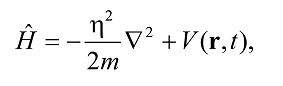
where the first term on the right-hand side represents the kinetic energy and the second term the potential energy related to some conservative external field V = V(r, t) which is a function of position and time. The ∇2 operator is a ‘smoothing operator’. The value of ∇2F(x, y, z) is the average of the values F(x, y, z) takes in some neighborhood of (x, y, z). To appreciate this point, recall that the solutions F(x, y, z) to Laplace’s equation ∇2F(x, y, z) = 0 are so analytically smooth that they possess derivatives of every order.
A reader new to quantum chaos can start with Barry Cipra61. The paper describes conjectural links between the Riemann zeta function related to prime numbers, and chaotic quantum-mechanical systems, and then read Martin Gutzwiller62 who produced a key formula, called a trace formula that showed how classical chaos might relate to quantum “chaos”. Gutzwiller is credited with the first investigation of relations between classical and quantum mechanics in chaotic systems.
Intriguing complexity. Finally, it is intriguing that the state vector |Ψâ© by postulate 1 is a complex entity with real and imaginary parts. While complex functions do appear in classical physics, they are invariably interpreted either as (1) an indicator that the solution is unphysical, e.g., in the Lorentz transformation when the speed of a physical object is greater than the speed of light, or (2) as a shortcut to dealing with two independent and equally valid solutions of the equations, one labelled real and the other imaginary, as in the case of two dimensional inviscid flow governed by the Laplace equation where the stream function and the velocity potential appear jointly as a complex variable. In quantum mechanics, |Ψâ© as a whole rather than its real and imaginary parts separately, is of interest. Yet, since |Ψâ© is not directly observable and is not a real physical entity, its complex character can be ignored, especially in view of postulate 3, which, in any case extracts a real value in a measurement. All measurable quantities depend on the absolute squares of the components of the state vector and such absolute squares are always real. At the quantum level, why does Nature prefer Hilbert space and complex variables? Why is √(-1) so central to Nature? We do not know.
[54] Wootters & Zurek (1982); Peres (2002) (As Asher reports, the title of the paper was contributed by John Wheeler.)
[55] Pati & Braunstein (2000).
[56] Braunstein & Pati (2007); Pati (Undated).
[57] Peres & Terno (2004).
[58] Luo, et al (2017).
[59] Pool (1989).
[60] Churchill (1939). The phrase is an adaptation of Winston Churchill’s remark about Russia during World War II: “It is a riddle wrapped in a mystery inside an enigma”.
[61] Cipra (1999).
[62] Gutzwiller (1990).
The brain is the only kind of object capable of understanding that the cosmos is even there, or why there are infinitely many prime numbers, or that apples fall because of the curvature of space-time, or that obeying its own inborn instincts can be morally wrong, or that it itself exists.63 —David Deutsch
Why Nature conforms to the above four postulates at the quantum level, and how they may link to the laws of classical physics (Newton’s laws of motion, Maxwell’s equations of electromagnetism, and Einstein’s theory of general relativity) has confounded the human mind. Yet, a strong belief in Bohr’s “correspondence principle” lingers that such a link would eventually emerge in the limit when the quantum numbers describing the system are large, meaning either some quantum numbers of the system are excited to a very large value, or the system is described by a large set of quantum numbers. For the present, the gulf between classical physics and quantum physics, as seen from Sections 2 and 3, appear so wide as to be unbridgeable. Even Bohr was pessimistic:
The repeatedly expressed hopes of avoiding the essentially statistical character of quantum mechanical description by the assumption of some causal mechanism underlying the atomic phenomena and hitherto inaccessible to observation would indeed seem to be as vain as any project of doing justice to the increased profundity of the picture of the world achieved by the general theory of relativity by means of the ordinary conceptions of absolute space and time. Above all such hopes would seem to rest upon an underestimate of the fundamental differences between the laws with which we are concerned in atomic physics and the every day experiences which are comprehended so completely by the ideas of classical physics.64
Recently, Peter Renkel with remarkable insight has hypothesized a bridge. He “starts from the generalization of a point-like object and naturally arrives at the quantum state vector of quantum systems in the complex valued Hilbert space, its time evolution and quantum representation of a measurement apparatus of any size. … [He shows] that a measurement apparatus is a special case of a general quantum object. [Finally, he provides an] example of a measurement apparatus of an intermediate size .”65
Modern information theory is based on two important facts: Shannon’s definition of information, and Landauer’s observation that information is physical because it must always be encoded in a physical system without which it is impossible to store, transmit, process, or receive information. Further, the information held by a physical system contributes to defining the state of the system. Note also, that in a mathematical (and hence a computational) model of the laws of Nature, semantic aspects are irrelevant to the interpretation problem. Nature can exist without humans interpreting it!
Shannon’s famous twin papers, A Mathematical Theory of Communication,66 published in July, October 1948, set the foundation for information theory. His seminal contribution was to define the concept of information mathematically, and then to consider the transmission of information as a statistical phenomenon in a way that gave communications engineers a method to determine the capacity of a communication channel in terms of classical bits. We know that information can be expressed and encoded in different but equivalent ways without losing its essential nature. The binary form allows convenient automatic manipulation of information: a computer need only manipulate quite simple things like integers to do surprisingly powerful information processing, from document preparation to differential calculus, to translating between human languages, to even mimicking human intelligence. Translation allows us to choose suitable hardware and software technologies for information processing.
Shannon also defined the crucial concept of information entropy (now called Shannon entropy)67 H(X) analogous to thermodynamic entropy:

which provides a way to estimate the average minimum number of bits needed to encode a string of symbols, based on the frequency of the symbols or the probability pi of its appearance. Shannon entropy does not measure degree of accuracy, it measures the degree of degeneracy of a system. In general, a complicated set of instructions can be reduced to n binary choices. We then have a ready measure of the information content of the object by simply counting the number of binary choices or the state of n binary bits. The state of a binary bit, by previous agreement, can be arbitrarily mapped to the binary alternatives, such as, 0 for spin-down of an electron and 1 for spin-up. We can thus use the bit as the unit of information and measure the information content of an information carrying object as the size of the set of instructions needed to reconstruct the state of the object.
In 1961, Rolf Landauer, in a seminal paper on reversible computing68, provided a remarkable insight. Since information is physical, a fact recently verified experimentally,692 the laws of physics must therefore place limits on information processing whether classical or quantum. He insightfully turned to thermodynamics and proved that only logically irreversible operations — those which cause information loss — expend energy. He showed that there is a fundamental asymmetry in the way Nature processes information. He proved the counter-intuitive result that all, but one, operation required in computation could, in principle, be performed in a reversible manner without dissipating heat. For example, copying classical information can be done reversibly and without wasting any energy, but when information is erased there is a minimum energy cost of kT ln 2 per classical bit (about 3 ï´ 10ïÂ21 joule at room temperature) to be paid, where k is the Boltzmann constant, and T is the absolute temperature in Kelvin of the computer’s environment. That is, the erasure of information is inevitably accompanied by the generation of heat. Once a system undergoes an irreversible action, its past history, unless archived, is irrevocably lost.
Landauer saw computations as engines converting free energy into waste heat and mathematical work where erasure of information inevitably leads to heat generation. For a lucid explanation of the erasure principle, see Plenio and Vitelli70. For experimental support of Landauer’s principle, see Orlov, et al71. Landauer’s principle and the second law of thermodynamics can indeed be understood as a logical consequence of the underlying reversible laws of physics as seen in the general Hamiltonian formulation of mechanics and in the unitary time evolution in quantum mechanics. Thus, Landauer’s principle connects physics with information theory. The connection led people to think of energy-efficient algorithms at a time when reducing algorithmic complexity was the craze.
What is remarkable about Landauer’s principle is that while computation is “an abstract mathematical process, mapping one set of input bits into another set of output bits”72, it is not at all obvious that there exists a fundamental connection between such a mapping and microscopic motion associated with heat. It, indeed, appears remarkable that logical reversibility of a computation (i.e., inputs can be inferred from the outputs) also implies physical reversibility73. The key to physical reversibility is to ERASE WITH A COPY.74 That information is convertible into energy has been experimentally shown.75
When Landauer published his paper, it was generally assumed that deterministic computation is not necessarily logically reversible and typical programming is unlikely to be so. Lecerf (1963) 76and Charles Bennett (1973)77 showed that deterministic computation could be simulated by a logically reversible Turing machine. That is, “it is possible to reprogram any deterministic computation as a sequence of logically reversible steps, provided the computation is allowed to save a copy of its input.” 78Bennett further suggested computing with nucleic acids to realize physical reversibility.79
By analogy with thermodynamics, one may conclude that Information that has not been compacted to reveal a useful interpretable pattern is random information, which on average does not create useful knowledge in a human mind. In this respect, molecular biologists face an acute problem. Till they find a theory to generate a given DNA sequence, the only way to communicate complete genetic information to another is to send the entire DNA sequence. On the other hand, the equations of physics have continually progressed towards compactness to an amazing degree. Physics is coded and computable information. Gregory Chaitin had the remarkable insight at a very young age that
a scientific theory is a computer program that calculates the observations, and that the smaller the program is, the better the theory. If there is no theory, that is to say, no program substantially smaller than the data itself, considering them both to be finite binary strings, then the observations are algorithmically random, theory-less, unstructured, incomprehensible and irreducible.80
To Chaitin, theory and computations are intimately connected:
theory = program –> Computer –> output = experimental data
[63] Deutsch (2012).
[64] Bohr (1937).
[65] Renkel (2017).
[66] Shannon (1948).
[67] Shannon, undecided whether to name his logarithmic formula ‘information’ or ‘uncertainty’, asked John von Neumann, who responded: Neither, and suggested: “You should call it entropy, for two reasons. In the first place your uncertainty function has been used in statistical mechanics under that name, so it already has a name. In the second place, and more important, no one really knows what entropy really is, so in a debate you will always have the advantage.” Source: Shannon’s Information Theory. Science4All, 17 March 2013. https://www.science4all.org/article/shannons-information-theory/
[68] Landauer (1961).
[69] Toyabe, et al (2010a, b).
[70] Plenio & Vitelli (2001). See also: Bennett (2003, revised 2011).
[71] Orlov, et al (2012).
[72] Orlov, et al (2012).
[73] Orlov, et al (2012).
[74] Orlov, et al (2012).
[75] Toyabe, et al (2010a, b).
[76] Lecerf (1963).
[77] Bennett (1973). A seminal contribution.
[78] Bennett (2003, revised 2011).
[79] Bennett. (1973). See also: Bennett. (1982); Thachuk (2013).
[80] Chaitin (2003).
In his classic 1985 paper titled ‘Quantum Theory, the Church-Turing Principle and the Universal Quantum Computer’81, David Deutsch described how a computer might run using the strange rules of quantum mechanics and why such a computer would differ fundamentally from ordinary computers. In fact, Deutsch showed that it is possible to construct reversible quantum gates for any classically computable function and suggested that quantum superposition might allow quantum evolution to perform many classical computations in parallel. Deutsch’s paper described the first true quantum Turing machine (QTM). In QTM, read, write, and shift operations were all accomplished by quantum mechanical interactions and whose “tape” could exist in states that were highly non-classical. For example, it could simultaneously encode many inputs to a problem on the tape and perform a calculation on all the inputs at the same time (quantum parallelism). In 1997, Samuel Bernstein and Umesh Vazirani82 showed that it is possible to conceive of a universal quantum Turing machine. In such a construction we must assume a sufficient supply of bits that correspond to the tape of a Turing machine. The QTM is sufficiently simple and at the same time universal to prove various theorems about quantum computation.
The universal quantum computer can perfectly simulate the UTM82. In addition, it can simulate various physical systems, real and theoretical, which are beyond the scope of the UTM. In quantum computers, we manipulate its global state at all times even when our intention is to manipulate a specific part of it, even as small as a qubit.
It is not yet clear if an equivalent of the Church-Turing Thesis exists for quantum computers. In 1985, David Deutsch provided a physical version of the Church-Turing Thesis: “Every finitely realizable physical system can be perfectly simulated by a universal model computing machine operating by finite means”. He then generalized the Thesis to “every computation, which can be realized physically, can be executed using a quantum Turing machine.”84 Deutsch has played a pioneering role in bringing quantum computing into the mainstream of computing.
To me quantum computation is a new and deeper and better way to understand the laws of physics, and hence understanding physical reality as a whole. — David Deutsch
The most important application of quantum computing in the future is likely to be a computer simulation of quantum systems, because that’s an application where we know for sure that quantum systems in general cannot be efficiently simulated on a classical computer. — David Deutsch
We do not know if quantum computers are inherently more powerful than classical computers partly because we are unsure how the quantum and the classical worlds are separated. For example, are there resources, truly unavailable in a classical world, being utilized in a quantum computation? It may eventually turn out that quantum computers are only as powerful as classical computers: that any problem which can be efficiently solved on a quantum computer can also be efficiently solved on a classical computer. It all depends on how clever we are in designing algorithms and the nature of algorithms permitted by the axiomatic systems we use in designing them. Also, there are issues of computability (i.e., which computational problems computers can or cannot solve), and issues of complexity (how efficiently computers can solve the problems they can). The fact that a computer can solve a particular kind of problem, in principle, does not mean that it can be done in practice for such obvious reasons that the running time of the computer is too long or the memory requirements are enormous, and so on.
In physics, the notion of space is intimately related to distribution of matter; two material objects cannot occupy the same space at the same time. The notion of time comes from change. Without detectable change there is no need for the notion of time. In mathematics there are two basic entities: operands (nouns) and operators (verbs). For an operand (noun) to change its value it needs to be operated on (verbed). Operands have space-like property in that they can move to a new value. Operators have time-like property because they bring about change. Operators may also show space-like properties as when describing the gradient of a distribution of operands. In natural languages too, we find certain nouns also used as verbs and vice versa. In quantum mechanics, operators serve as surrogates for certain operands, hence commutability of operators plays such an important role in measurement. Here are a few such operators:
[81] Deutsch (1985).
[82] Bernstein & Vazirani (1997).
[83] Deutsch (1985).
[84] Deutsch (1985).
In quantum mechanics, vectors in a vector space describe states of a quantum system. The state vector carries both classical and quantum information. The classical information is accessible to classical measurement, the quantum information is not. The state space of a composite quantum system is the tensor product of individual Hilbert spaces H = H1 H2. If the state of a composite system cannot be written as |Ψ⟩ = |Ψ1⟩ ⊗ |Ψ2⟩ of its components, it is an entangled state.
Finally, when working with vectors in an n-dimensional vector space, it is extremely useful to have a set of n mutually orthogonal unit vectors and use them as the basis (orthonormal basis) to construct any vector in that space. Such a vector will necessarily be a linear combination of the basis vectors. In fact, the dimension of the vector space can be defined as the maximum number n of mutually orthogonal vectors that can be found in that space. An orthonormal basis is not unique, but n is. Any two bases can be related to each other for conversion purposes. For example, one may choose one basis for preparing a quantum system but measure it in another basis. Specifying an orthonormal basis is conceptually similar to choosing a Cartesian coordinate system in physical three-dimensional space.
Any extraction of a real measurable variable from an abstract entity requires some transformative operator. Such operators acting on |Ψ⟩ are called observables in the literature. To make it explicit, in this paper we call them “observable-operators”. In classical physics, the measurable information is directly available, in quantum mechanics it is not. This is a crucial difference. A quantum observable-operator, is an intermediary that produces a classical value when it acts on |Ψ⟩. The operator’s unusual action is that it initiates the random “collapse” of |Ψ⟩ to one of the operator’s eigenvectors according to postulate 3. Further, the classical value the operator produces is the eigenvector’s corresponding eigenvalue.
Observable-operators arise in quantum mechanics because it deals with probability waves (the state vector) rather than with discrete particles whose motion and dynamics can be deterministically described by Newtonian physics. Part of the development of quantum mechanics is the establishment of the operators associated with the parameters needed to describe the system.
Recall that Fig. 3.1 could be interpreted in two ways. That picture, a classical object, did not capture the irreversible aspect of quantum measurement, nor can we claim that the state we observed is an eigenstate. The picture collapses to an interpretation (from the observer’s point of view) or flickers only during the observed period and stays superposed at other times. We infer this because we believe the picture is a static object. Thus, any observation is independent of all other observations. Further, more than one observer can observe the picture concurrently, each making his own interpretation. Thus, multiple observers, in principle, can pool their observations and determine all the possible states of the picture. In quantum mechanics, such pooling is not possible.
Modern scientific theories seek confirmation in observations.85 Observations require that some external agency interact with the system being measured. Measurements must follow a strict protocol to minimize disturbance to the measured object. We hope that the measured system can tolerate some minimum disturbance without getting destabilized to enable observations. A classical measuring apparatus always destabilizes a quantum system. Hence, we cannot expect to find any deterministic causal connections using measurements. However, we may assume causality to apply to undisturbed systems, e.g., we may express the evolution of the system (or subsystem) by differential equations that relate past conditions with future ones, but their ability to connect with observations will only be indirect; there will be an unavoidable indeterminacy in the calculation of observational results.
Physical measurements produce real numbers, so we are concerned with real dynamical variables. A complex dynamical variable necessitates two measurements—one each for the real and imaginary parts. This works fine only when measurements introduce negligible disturbances in the measured system (as in classical fluid flows where complex variables are sometimes used).86 In quantum systems, when Heisenberg’s uncertainty principle applies, one cannot make simultaneous measurements if non-commutating observable-operators are involved. Further, the sequence in which the variables are measured, matters. Observables are also associated with a vector space, but they are not state-vectors. They are the things we measure, and they are represented by linear operators.87
In quantum mechanics, measurements are intimately related to the eigenvalues and eigenvectors of observable-operators. In fact, the eigenstates have a significance beyond that of an orthonormal basis. Every measurable quantity, by postulate, has an associated observable-operator represented by a Hermitian operator and not a variable! A Hermitian operator M, has the defining self-adjoint property, i.e., M = M†. (The complex conjugate of a transposed matrix is called its Hermitian conjugate, denoted by a dagger superscript.) The set of eigenvalues of M represents the set of measurement outcomes M can produce. Each eigenvalue has a corresponding eigenstate (or eigenvector), to which the system will collapse after the measurement.
Note also that
The above implies that any state of a quantum system can be expressed as a linear combination of the eigenvectors of any Hermitian operator. Equivalently, it means that any quantum state can be expressed as a linear superposition of the eigenstates of an observable-operator. Classical mechanics deals with real variables, quantum mechanics deals with operators whose eigenvalues are real. When the focus is on operators whose fundamental property is to bring about change is it surprising that quantum mechanics needs a separate postulate for measurement, while classical mechanics, which ideally views measurement as a passive activity, does not?
A complicated situation arises when there are two or more eigenstates of an observable with the same eigenvalue. Then any state formed by the linear superposition of the eigenstates will also be an eigenstate of the observable-operator belonging to the same eigenvalue. The implication here is that if two or more states for which a measurement of the observable is certain to belong to the same eigenvalue, then for any state formed by superposition of them will also belong to the same eigenvalue. This means that it is always possible to find two orthogonal vectors to form linear combinations.88 Since two eigenstates of an observable-operator attached to different eigenvalues are orthogonal, it follows that two states for which a measurement is certain to give two different results are orthogonal too.
[85] Aristotle (384 BC – 322 BC) did not seek confirmation in observations nor did he think it was necessary. Galileo (1564-1642) decidedly thought otherwise while laying the foundation for modern physics.
[86] See, e.g., Lamb (1932).
[87] Susskind & Friedman (2015), Chapter 3, Sec. 3.1.1.
[88] Susskind & Friedman (2015), Chapter 3, Sec. 3.1.5.
Note that while we cannot speak of an observable having a value for a particular state, we can speak of the probability of its having any specified value for the state (i.e., the probability of it being obtained when one makes a measurement) and we can define an average value for the state. It is permissible for a quantum state to be simultaneously an eigenstate of two observables; the chances for such an existence are most favorable if the two observables commute and rather exceptional when they do not. When the observables commute, there exist so many simultaneous eigenstates that they form a complete set.89 The case when two observables commute is special in the sense that the observations are non-interfering or compatible in such a way that one can give a meaning to the two observations being made simultaneously and discuss the probability of their being obtained. Indeed, one may view the two observations as a single observation of a more complicated type, the result of which is two real numbers rather than one. A natural generalization of this is that any two or more commuting observable-operators may be treated as a single observable-operator whose action produces two or more numbers. The states for which this measurement is certain to lead to one particular result are the simultaneous eigenstates.
After measurement, the system remains in its collapsed state unless altered. Till altered, any repetition of the measurement will only reproduce the first measurement. This is the deep connection between the set of eigenvalues of an observable-operator and the possible results of measurement associated with that observable-operator. One may, of course, alter the post-measurement state of the system by measuring a different observable or measuring in a different basis or by applying a quantum (unitary) operation.
Global phase factor
Consider the state eiϒiϒ|Ψ⟩ is equal to |Ψ⟩, up to a global phase factor eiϒ. What is interesting is that the measurement statistics predicted for these two states are identical. To see this, suppose Mm is a measurement operator associated to some quantum measurement, then the respective probabilities that an outcome corresponding to index m will occur are
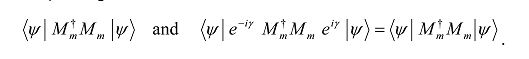
Thus, from a measurement point of view the two states are identical and global phase factors are irrelevant to the observed properties of physical systems. This symmetry, of all things, implies the conservation of electric charge in the Universe!90
Relative phase factor
Consider the states a|0⟩ + b|1⟩ and c|0⟩ + d|1⟩. We say that two complex amplitudes, such as, a and c differ by a relative phase factor if there is a real θ (relative phase shift) such that a = eiθc. We likewise say that complex amplitudes b and d differ by a relative phase factor if there is a real ∅ such that b = ei∅d. Note that θ and ∅ depend on the basis being used to represent the states.
Example. In the two states (1/√2) (|0⟩ + |1⟩) and (1/√2) (|0⟩ – |1⟩), the amplitudes of |0⟩ are the same in the two states, hence they have a relative phase factor of 1, while the amplitudes of |1⟩ differ by a relative phase factor of -1.
The difference between the relative phase factors and global phase factors is that for relative phase the phase factors may vary from amplitude to amplitude, which makes the relative phase a basis-dependent concept unlike the global phase. As a result, states, which differ only by relative phases in some basis, give rise to physically observable differences in measurement statistics, and it is no longer possible to regard these states as being physically equivalent.
A matrix or an operator U is unitary if U† U = I. An operator is unitary if and only if each of its matrix representations is unitary. U is invertible, normal, and has a spectral decomposition (i.e., it can be diagonalized), and preserves inner products between vectors. Each eigenvalue of a unitary matrix has modulus 1 (i.e., it has the form eiθ for some real θ). The tensor product of two unitary operators is unitary. Unitarity simply means the equality of two lengths. Any unitary transformation is equivalent to a rotation, and an L2 length that remains invariant to a rotation. A L2 length has the form of a sum of squares.
Rather surprisingly, the unitarity constraint is the only constraint required of quantum gates. Thus, any unitary matrix specifies a valid quantum gate! Further, it can be shown that any arbitrary 2×2 unitary matrix may be decomposed as
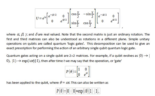
Quantum computing uses unitary operators to change the state of discrete state vectors when that change is being made under postulate 2. This change can be reversed by the corresponding inverse operator (which always exists) if it is applied before any measurement is made on the quantum system. Reversible operators (gates) only move states around; they have the same number of inputs and outputs and have a one-to-one mapping between input vectors and output vectors. Every reversible gate can be described by a permutation. Thus, a reversible operator’s input and output are uniquely retrievable from each other. As no information is lost, energy is conserved. Finally, since the evolution of a quantum system is governed by unitary operators, non-unitary operations (such as irreversible operations) are not admissible when operating under postulate 2. Thus, quantum gates do not allow (1) feedback loops from one part of the system to another, (2) fan-in operations (that is, bitwise OR of inputs), and (3) fan-out operations (because it would violate the no-cloning theorem).
We now look at some qubit transformations (gates) which are central to quantum computing. The reader should commit these transformations to memory and become familiar with their use. The 1-qubit transformations (gates), namely the Pauli gates, and the Hadamard gate, and the 2-qubit Cnot gate are particularly important. They are all unitary matrices. In matrix form, by convention, the basis states are lexicographically ordered, e.g., 3-qubit gates are ordered according to |000⟩, |001⟩, |010⟩, |011⟩, |100⟩, |101⟩, |110⟩, and |111⟩.
Pauli gates
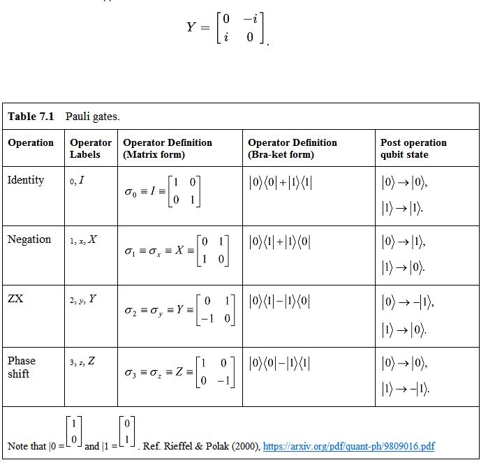
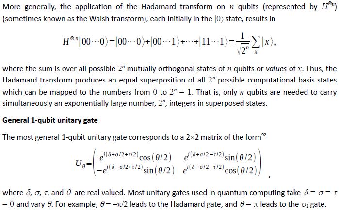
In quantum computing, Pauli gates (also called σ-matrices), named after Wolfgang Pauli who won the 1945 Nobel Prize in physics for his “decisive contribution through his discovery of a new law of Nature, the exclusion principle or Pauli principle”, play a central role in the manipulation of single qubits. They are represented by 2×2 matrices as shown in Table 7.1. Except for I, all have trace zero. Some authors do not include I in the set of Pauli matrices (also called σ-matrices). We will include I. Any 2×2 matrix M can be expressed as the linear sum M =α I +β X + γY + δZ, where α,β ,γ ,δ are complex constants. Thus, there are infinitely many 2×2 unitary matrices, and therefore infinitely many single qubit gates, but each is expressible as linear combinations of the matrices, I, X, Y, and Z. This contrasts with classical information theory, where only two logic gates are possible for a single bit, namely the identity and the logical NOT operation.
[90] See, e.g., Peskin & Schroeder (1995), Section 7.4 (“The Ward-Takahashi identity”).
[91] A half-silvered mirror effects this transformation on a photon when it encounters the mirror.
Note: The Y gate is often represented in the alternate form where it maps |0⟩ to i|1⟩ and |1⟩ to i|0⟩, which in matrix form appears as
Some frequently used gates 1-qubit gates
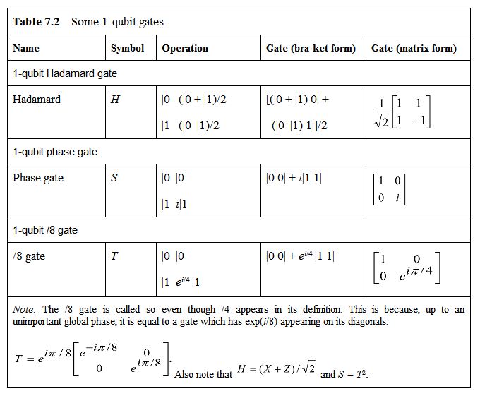
The Hadamard gate, the phase gate, and the π/8 gate are frequently used gates. They are shown in Table 7.2. The Hadamard gate is frequently used in quantum computations as the first step in creating input data at the start of computations. It is a special case of the more general Fourier transform. It transforms a qubit in state |0⟩ into the superposed state H|0⟩ = (|0⟩ + |1⟩)/√2≡ |+⟩ and likewise state |1⟩ into H|1⟩ = (|0⟩ |1⟩)/√2≡|-|⟩.91 That is, H rotates the state of a qubit (remember unitary operators only rotate a state vector) such that the result may also be viewed as just a change in basis:
(|0⟩, |1⟩) → (|+⟩, |-⟩).91
The result is that if the qubit is measured in the basis, after being operated by the Hadamard gate, we will get |0⟩ or |1⟩ with equal probability, but if it is measured using the (|+⟩, |-⟩) basis, we will measure |+⟩ if the qubit’s earlier state was |0⟩ and |-⟩ if the qubit’s earlier state was |1⟩ . Note that H is its own inverse, or H2 = I, that is, applying H twice to a state does nothing to it, and this is amazing; by applying a randomizing operation to a random state produces a deterministic outcome! Of course, only under the laws of quantum mechanics and not of classical mechanics. The (|0⟩, |1⟩) and (|+⟩, |-⟩) the bases are among the most frequently used bases in quantum computing, hence the reader should instinctively think about them when designing a new algorithm, especially as the first step in the algorithm for inputting all possible input data.
2-qubit controlled-not gate
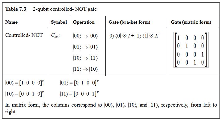
The 2-qubit controlled-not gate, Cnot, is a generalization of the irreversible classical XOR gate. Here the state of the bit chosen as the control bit decides what happens to the other called the target bit as described below. Let |a⟩⊕|b⟩≡|a,b⟩ represent a 2-qubit system on which it acts. Then, if the first bit is the control bit,
Cnot |a,b⟩ = |a, a ⊗b⟩
where ⊕ signifies the exclusive-or (XOR) operation (i.e., modulo 2 addition)93. It means that the output is “true” if and only if exactly one of the operands has a value “true”. This gate cannot be decomposed into a tensor product of two 1-qubit transformations, that is, one cannot find two unitary operators O1 and O2 such that Cnot = O1 ⊗ O2. The list of state changes shown in Table 7.3 is the analog of the truth table for a classical binary logic gate. Note that |00⟩, |01⟩, |10⟩, |11⟩ form an orthonormal basis for the state space of a 2-qubit system. By convention they are associated to the standard 4-tuple basis as shown in Table 7.3.
The resulting states are known as the Bell states (after John Bell) or sometimes as the EPR states or EPR pairs (after Einstein, Podolsky, and Rosen of the EPR-paradox fame; see Section 4.2). They are unique because they are all entangled states, i.e., in an unfactorizable state. When entangled particles are used to encode bits, their joint state represents an ebit.
Unlike a classical bit or a qubit, an ebit is, intrinsically, a shared resource. The information an ebit carries is always distributed between two particles. Hence the states of these particles are correlated, but undetermined until measured. An ebit therefore provides the basis for a restricted kind of quantum communication channel in the sense that once either particle comprising the ebit is measured, the state of both particles becomes definite. However, the channel is restricted in the sense that you cannot send an intentional message between two parties simply by having each party measure his or her members of a set of shared ebits, because, individually, the sequence of results (the decoded bits) would appear random.
Toffoli gate
The quantum Toffoli gate95 is a 3-qubit gate with three bits in and three bits out. A combination of 1-qubit unitary operations and a single 2-qubit operation (Cnot) is sufficient to build this gate. It can be viewed as a controlled-controlled-NOT gate, which negates the last of three bits if and only if the first two are 1, i.e., T |a, b, c⟩ = | a, b, c⊕ ab⟩. The Toffoli gate, applied twice to a set of bits has the effect (a, b, c) → (a, b, c⊕ ab) → (a, b, c). Thus, the Toffoli gate is reversible, since it is its own inverse. The use of three qubits is necessary to permit the whole operation to be unitary.

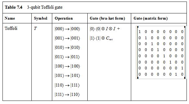
The 3-qubit Toffoli gate can be used to construct a complete set of Boolean connectives. In support of this statement, the AND and NOT operators are shown below:
T |x, y, 0⟩ = |x, y, x ∧ y⟩.
T |1, 1, x⟩ = |1, 1,¬x⟩.
The classical Toffoli gate is, therefore, a classical universal gate. The quantum version, which simply permutes computational basis states in the same way as the classical Toffoli gate, nevertheless cannot carry out the FANOUT operation because of the no-cloning theorem. The quantum Toffoli gate is not a universal gate in quantum computing, but it can implement all possible classical computations on a quantum computer. The Toffoli gate allows the irreversible classical gates to become reversible. This means that quantum computers can mimic the Universal Turing Machine despite being restricted to reversible, unitary gates.
Classical computers compute using Boolean expressions. Any Boolean expression may be constructed from a non-unique set of universal logic gates. For example, the AND, OR, and NOT gates form a universal set. Alternatively, AND and NOT (also known as NAND), or OR and NOT or AND and XOR form three other possible universal sets. In addition to gates, one needs extra ancilla or working bits, to allow extra working space during computations. Muller’s theorem96 tells us that the choice of a universal set has little effect on the complexity of computing. Note that the operations of AND, OR, and XOR gates are many-to-one. Therefore, they are logically irreversible. Only the NOT gate is reversible since it is a one-to-one operation. Clearly then, the information content on the right-hand side of
(a, b) → NOT (a AND b)
is less than on the left-hand side.
Any unitary operation on n qubits can be implemented exactly by stringing together operations composed of single qubit and controlled-NOT gates97. For example, the Hadamard, phase98, controlled-NOT, and /8 gates provide a set of universal gates for which fault-tolerant constructions are known. This set is the standard set of universal gates. There is a second set of universal gates comprising the Hadamard, phase, controlled-NOT, and Toffoli gates, which may also be constructed in a fault-tolerant manner. We omit the proofs. In fact, there are many more choices for the universal quantum gate than in classical reversible computing due to the greater power of quantum computing. For example, DiVincenzo99 showed that two-qubit universal quantum gates are indeed possible and Barenco100 extended this knowledge to show that almost any two-qubit (within a certain restricted class) is universal. Subsequently, Lloyd101 and Deutsch, et al102, have shown that almost any two-qubit or n-qubit (n≥2) quantum gate is also universal.
Once Rolf Landauer,103 Charles Bennett104, Tommaso Toffoli,105 Edward Fredkin106 and others showed that reversible computing on a Turing machine was indeed possible and computationally economical, it was clear that quantum computers can simulate Turing machines by ensuring that they remain in a computational basis state at the end of each step, given that they start in one. To ensure unitarity, it is necessary and sufficient that the mapping from one state to another be bijective. In fact, the universal quantum computer can perfectly simulate107 any Turing machine and can simulate with arbitrary precision any quantum computer or simulator. In principle, any quantum particle, e.g., a photon or an electron, can function as a gate. The idea that quantum computers can be built to perform any computation reversibly both logically and thermodynamically by a physical apparatus dissipating arbitrarily little energy108 is no longer a fantasy.
Thus far we have explained certain fundamental differences between classical and quantum physics. We have emphasized that these differences require unusual approaches to algorithmic problem solving when using quantum computers. In Section 7 we concluded Part I by describing a set of core unitary quantum operators required to manipulate the state vector of a quantum computer. We will use these operators extensively in Part II to develop an array of quantum algorithms for general problem solving.
[91] A half-silvered mirror effects this transformation on a photon when it encounters the mirror.
[92] Braunstein (1995).
[93] In modulo 2 arithmetic, the following addition rules for adding two binary numbers are quite obvious:
0 + 0 ≡ 0 (mod 2), 0 + 1 ≡ 1 (mod 2), 1 + 0 ≡ 1 (mod 2), 1 + 1 ≡ 0 (mod 2).
Analogously, the XOR (or Cnot) operation is: 0 ⊗ 0 = 0, 0 ⊗ 1 = 1, 1 ⊗ 0 = 1, 1 ⊗ 1 = 0.
[94] See Barenco, et al (1995).
[95] Toffoli (1980). It is named after Tommaso Toffoli, who in 1980 showed that the classical version is universal for classical reversible computation.
[96] Muller (1956).
[97] See, e.g., Nielsen and Chuang (2000), pp. 189 and 191.
[98] Though the phase gate, S = T2, it is included because of its natural role in the fault-tolerant constructions.
[99] DiVincenzo (1995).
[100] Barenco (1995).
[101] Lloyd (1995).
[102] Deutsch, Barenco & Ekert (1995), pp. 669-677.
[103] Landauer (1961).
[104] Bennett (1982).
[105] Toffoli (1980).
[106] Fredkin & Toffoli (1982).
[107]Deutsch, D. (1985), p. 107.
[108] See, e.g., Landauer (1961), and Bennett (1973). Bennett, in particular, showed that a Turing machine “may be made logically reversible at every step, while retaining their simplicity and their ability to do general computations.” He also discussed the biosynthesis of messenger RNA as a physical example of reversible computation.
Cited URLs were last accessed on 31 January 2018.
[1] Aaronson (2013). Aaronson, S. The Ghost in the Quantum Turing Machine. arXiv:1306.0159v2 [quant-ph], 07 June 2013. https://arxiv.org/abs/1306.0159
[2] Abbott, et al (2016). Abbott, B. P., et al. Observation of Gravitational Waves from a Binary Black Hole Merger. Physical Review Letters, PRL 116, 061102, 2016. https://physics.aps.org/featured-article-pdf/10.1103/PhysRevLett.116.061102
[3] Al-Kahlili (2003). Al-Kahlili, J. Quantum. Weidenfeld & Nicolson, London, 2003.
[4] Aspect (1991). Aspect, A. Testing Bell’s Inequalities. Europhys. News, 22, 73-75, 1991. https://www.europhysicsnews.org/articles/epn/pdf/1991/04/epn19912204p73.pdf
[5] Aspect, Dalibart & Roger (1982). Aspect, A., Dalibart, J., and Roger, G. Experimental Test of Bell’s Inequalities Using Time-Varying Analysers. Physical Review Letters, 49, 1804-1807, 1982. https://journals.aps.org/prl/pdf/10.1103/PhysRevLett.49.1804
[6] Barenco, et al (1995). Barenco, A., et al. Elementary Gates for Quantum Computation. arXiv:quant-ph/9503016v1, 23 March 1995. https://arxiv.org/pdf/quant-ph/9503016v1.pdf Also as: Barenco, A., Bennett, C.H., Cleve, R., DiVincenzo, D.P., Margolus, N., Shor, P., Sleator, T., Smolin, J.A., and Weinfurter, H. Elementary Gates for Quantum Computation. Physical Review A, 52, 3457-3467, 1995.
[7] Bell (1964). Bell, J. S. On the Einstein-Podolsky-Rosen Paradox. Physics, 1, 195-200, 1964. http://inspirehep.net/record/31657/files/vol1p195-200_001.pdf (Reprinted in Bell, J. S. Speakable and Unspeakable in Quantum Mechanics, Cambridge University Press, Cambridge, 1987.
[8] Bennett (1973). Bennett, C. H. Logical Reversibility of Computation. IBM Journal of Research and Development, 17, 525–532, November 1973. https://www.math.ucsd.edu/~sbuss/CourseWeb/Math268_2013W/Bennett_Reversibiity.pdf
[9]Bennett. (1982). Bennet, C. H. The Thermodynamics of Computation – A Review. International Journal of Theoretical Physics, 21, 905–940, 1982. https://www.cc.gatech.edu/computing/nano/documents/Bennett%20-%20The%20Thermodynamics%20Of%20Computation.pdf. Reprinted in Leï¬ & Rex (1990). Leff, H. S., and Rex, A. F. (Eds). Maxwell’s Demon: Entropy, Information, Computing. Chapter 4, Sec. 4.2. CRC Press, 1990.
[10] Bennett (2003, revised 2011). Bennett, C. H. Notes on Landauer’s Principle, Reversible Computation, and Maxwell’s Demon. arXiv:physics/0210005v2 [physics.class-ph], 9 Jan 2003. https://arxiv.org/pdf/physics/0210005.pdf;
https://www.math.ucsd.edu/~sbuss/CourseWeb/Math268_2013W/Bennett_Reversibiity.pdf
[11] Bernstein & Vazirani (1997). Bernstein, E., and Vazirani, U. V. Quantum Complexity Theory. SIAM Journal on Computing, 26(5), 1411-1473, 1997. A preliminary version of this paper appeared in the Proceedings of the 25th ACM Symposium on the Theory of Computing, 1993.
[12] Bohm (1952). Bohm, D. A Suggested Interpretation of the Quantum Theory in Terms of “Hidden” Variables. Physical Review, 85, 166-193, 1952. http://fma.if.usp.br/~amsilva/Artigos/p166_1.pdf
[13] Bohm & Hiley (1993). Bohm, D., and Hiley, B. J. The Undivided Universe. Routledge, London, 1993.
[14] Bohr (1928). Bohr, N. The Quantum Postulate and the Recent Development of Atomic Theory. Naturwissenschaften, 16(15), 245-257, 1928. (Bohr’s Como lecture (delivered on 16 September 1927)). http://www.psiquadrat.de/downloads/bohr28_como.pdf
[15] Bohr (1934). Bohr, N. Atomic Theory and Description of Nature, 1. Cambridge, 1934.
[16] Bohr (1935). Bohr, N. Can Quantum-Mechanical Description of Physical Reality be Considered Complete? Physical Review, 48, 696-702, 1935. https://journals.aps.org/pr/pdf/10.1103/PhysRev.48.696
[17] Bohr (1937). Bohr, N. Causality and Complementarity. Philosophy of Science, 4 (3), 1937. http://www.informationphilosopher.com/solutions/scientists/bohr/Causality_and_Complementarity.pdf
[18] Born (1926a). Born, M. Zur Quantenmechanik der Stoßvorgänge. Zeitschrift für Physik, 37 (12), 863–867, 1926. http://www.psiquadrat.de/downloads/born26_stossvorgaenge.pdf
[19] Born (1926b). Born, M. Quantenmechanik der Stoßvorgänge. Zeitschrift für Physik, 38 (11-12), 803-827, 1926. English translation in Ludwig, G., (Ed.). Wave Mechanics, Pergamon Press, Oxford, 1968.
[20] Born (1954). Born, M. The Statistical Interpretation of Quantum Mechanics, Nobel Lecture, 11 December 1954, https://www.nobelprize.org/nobel_prizes/physics/laureates/1954/born-lecture.pdf
[21] Bose, et al (2017). Bose, S., et al. A Spin Entanglement Witness for Quantum Gravity. arXiv:1707.06050 [quant-ph], 19 July 2017, https://arxiv.org/abs/1707.06050
[22] Braunstein (1995). Braunstein, S. L., Quantum Computation, 1995. http://www-users.cs.york.ac.uk/~schmuel/comp/comp_best.pdf
[23] Braunstein & Pati (2007). Braunstein, S. L., and Pati, A. K. Quantum Information Cannot be Completely Hidden in Correlations: Implications for the Black-Hole Information Paradox. Physical Review Letters, 98 (080502), 2007. https://journals.aps.org/prl/abstract/10.1103/PhysRevLett.98.080502
[24] Byrne (2007). Byrne, P. The Many Worlds of Hugh Everett. Scientific American, December 2007. http://www.scientificamerican.com/article.cfm?id=hugh-everett-biography
[25] Chaitin (2003). Chaitin, G. J. Leibniz, Information, Math and Physics. arXiv:math/0306303v2 [math.HO], 21 Jun 2003. https://arxiv.org/pdf/math/0306303.pdf
[26] Churchill (1939). Churchill, W. The Russian Enigma. BBC Broadcast, 01 October 1939. http://www.churchill-society-london.org.uk/RusnEnig.html
[27] Cipra (1999). Cipra, B. A Prime Case of Chaos. What’s Happening in the Mathematical Sciences, 4, American Mathematical Society, 1999. http://www.ams.org/samplings/math-history/prime-chaos.pdf
[28] Deutsch (1985). Deutsch, D. Quantum Theory, the Church-Turing Principle and the Universal Quantum Computer. Proceedings of the Royal Society of London; Series A, Mathematical and Physical Sciences, 400 (1818), 97–117, 1985. http://www.qubit.org/oldsite/resource/deutsch85.pdf.
[29] Deutsch (1997). Deutsch, D. The Fabric of Reality. Penguin Books, New York, 1997.
[30] Deutsch (2009). Deutsch, D. A New Way to Explain Explanation. TEDGlobal 2009, July 2009. https://www.ted.com/talks/david_deutsch_a_new_way_to_explain_explanation
[31] Deutsch (2012). Deutsch, D. Creative Blocks. Aeon, 03 October 2012. https://aeon.co/essays/how-close-are-we-to-creating-artificial-intelligence
[32] Deutsch, Barenco & Ekert (1995). Deutsch, D., Barenco, A., and Ekert, A. Universality in Quantum Computation. Proceedings of the Royal Society of London A, 449, 669-677, 1995.
[33] Dirac (1939). Dirac, P. A. M. A New Notation for Quantum Mechanics. Mathematical Proceedings of the Cambridge Philosophical Society. 35 (3), 416–418, 1939. http://www.ifsc.usp.br/~lattice/wp-content/uploads/2014/02/Dirac_notation.pdf
[34] Dirac (1958). Dirac, P. A. M. The Principles of Quantum Mechanics, 4th Ed. Oxford University Press, 1958.
[35] DiVincenzo (1995). DiVincenzo, D. P. Two-bit Gates are Universal for Quantum Computation. Physical Review A, 50, 1015-1022, 1995. Also at https://arxiv.org/abs/cond-mat/9407022
[36] Einstein, Podolsky & Rosen (1935). Einstein, A., Podolsky, B., and Rosen, N. Can Quantum-Mechanical Description of Physical Reality be Considered Complete? Physical Review, 47, 777-780, 1935. https://journals.aps.org/pr/pdf/10.1103/PhysRev.47.777
[37] Everett (1957a). Everett, H. On the Foundations of Quantum Mechanics. Ph.D. thesis, Princeton University, Department of Physics, 1957.
[38] Everett (1957b). Everett, H. “Relative State” Formulation of Quantum Mechanics. Reviews of Modern Physics, 29 (3), 454-462, July 1957. http://www.univer.omsk.su/omsk/Sci/Everett/paper1957.html
[39] Everett (1963). Everett, H. Generalized Lagrange Multiplier Method for Solving Problems of Optimum Allocation of Resources. Operations Research, 11 (3), June 1963, 399 – 417, 1963. http://www.hpca.ual.es/~jjsanchez/references/Generalized_Lagrange_multiplier_method_for_solving_problems_of_optimum_allocation_of_resources.pdf
[40] Feynman (1965). Feynman, R.P. The Character of Physical Law. The Modern Library, New York, 1994. (Originally published by BBC in 1965.)
[41] Fredkin & Toffoli (1982). Fredkin, E., and Toffoli, T. Conservative Logic. International Journal of Theoretical Physics, 21, 219-253, 1982. http://calculemus.org/logsoc03/materialy/ConservativeLogic.pdf
[42] Gidney (2016). Gidney, C. Bra-Ket Notation Trivializes Matrix Multiplication. Algorithmic Assertions, 27 November 2016. http://algassert.com/post/1629
[43] Gutzwiller (1990). Gutzwiller, M. C. Chaos in Classical and Quantum Mechanics. Springer, New York, 1990.
[44] Handsteiner, et al (2017). Handsteiner, J., et al. Cosmic Bell Test: Measurement Settings from Milky Way Stars. Physical Review Letters, 118 (060401), 07 February 2017. https://journals.aps.org/prl/pdf/10.1103/PhysRevLett.118.060401
[45] Heisenberg (1927). Heisenberg, W. Über den anschaulichen Inhalt der quantentheoretischen Kinematik und Mechanik. Zeitschrift für Physik, 43 (3-4), 172-198, 1927. https://people.isy.liu.se/jalar/kurser/QF/references/Heisenberg1927.pdf English translation in (Wheeler and Zurek, 1983), pp. 62-84. Another English translation (The Actual Content of Quantum Theoretical Kinematics and Mechanics), available as NASA TM 77379 (December 1983) https://ia600500.us.archive.org/10/items/nasa_techdoc_19840008978/19840008978.pdf
[46] Heisenberg (1974). Heisenberg, W. Across the Frontiers. Harper & Row, New York, 1974.
[47] Hensen, et al (2015). Hensen, B. et al. Loophole-free Bell Inequality Violation using Electron Spins Separated by 1.3 kilometres. Nature, 526, 682–686, 29 October 2015. Preprint at https://arxiv.org/abs/1508.05949 (2015)
[48] Hilgevoord & Uffink (2016). Hilgevoord, J., and Uffink, J. The Uncertainty Principle, The Stanford Encyclopedia of Philosophy (Winter 2016 Edition), Edward N. Zalta (ed.). https://plato.stanford.edu/entries/qt-uncertainty/
[49] Jammer (1974). Jammer, M. The Philosophy of Quantum Mechanics. Wiley & Sons, New York, 1974.
[50] Kreyszig (2011). Kreyszig, E. Advanced Engineering Mathematics, 10th Ed. Wiley Plus, 2011. http://instructor.sdu.edu.kz/~merey/Advanced%20Engineering%20Mathematics%2010th%20Edition.pdf
[51] Laloë (2001). Laloë, F. Do We Really Understand Quantum Mechanics? Strange Correlations, Paradoxes, and Theorems. American Journal of Physics, 69 (6), 655-701, 2001. http://hal.archives-ouvertes.fr/docs/00/02/75/08/PDF/mq-anglais.pdf Correction at American Journal of Physics, 70, 556, 2002. http://aapt.scitation.org/doi/abs/10.1119/1.1466818
[52] Lamb (1932). Lamb, H. Hydrodynamics. Cambridge University Press, 1932.
[53] Landauer (1961). Landauer, R. Irreversibility and Heat Generation in the Computing Process. IBM Journal of Research and Development, 5 (3), 183-191, 1961. Reprinted in IBM Journal of Research and Development, 44 (1-2), 261-269, January/March 2000.
http://www.pitt.edu/~jdnorton/lectures/Rotman_Summer_School_2013/thermo_computing_docs/Landauer_1961.pdf
[54] Lecerf (1963). Lecerf, Y. Machines de Turing réversibles. Comptes Rendus Hebdomadaires des Séances de L’académie des Sciences, 257, 2597–2600, Séance du 28 Octobre 1963. http://vadeker.net/corpus/reversible/turing.html
[55] Lloyd (1995). Lloyd, S. Almost Any Quantum Logic Gate is Universal. Physical Review Letters, 75(2), 346-349, 1995. http://capem.buffalo.edu/rashba/p346_1.pdf
[56] Luo, et al (2017). Luo, M-N., Li, H-R., Lai, H., & Wang, X. Unified Quantum No-Go Theorems and Transforming of Quantum States in a Restricted Set. arXiv:1701.04166v2 [quant-ph], 19 March 2017, https://arxiv.org/pdf/1701.04166.pdf
[57] Marquardt & Püttmann (2008). Marquardt, F and Püttmann, A. Introduction to Dissipation and Decoherence in Quantum Systems. arXiv:0809.4403v1 [quant-ph] 25 September 2008. https://arxiv.org/pdf/0809.4403.pdf
[58] Merali (2015). Merali, Z. Toughest Test Yet for Quantum ‘Spookiness’. Nature, 525, 14-15, 03 September 2015
http://www.nature.com/polopoly_fs/1.18255!/menu/main/topColumns/topLeftColumn/pdf/nature.2015.18255.pdf
[59] Mermin (2004). Mermin, N. D. Could Feynman have Said This? Physics Today, 57 (5), 10-11, May 2004. http://physicstoday.scitation.org/doi/10.1063/1.1768652
[60] Muller (1956). Muller, D. E. Complexity in Electronic Switching Circuits. IRE Transactions on Electronic Computers, EC-5 (1), 15-19, March 1956.
[61] Nielsen & Chuang (2000). Nielsen, M. A., and Chuang, I. L. Quantum Computation and Quantum Information. Cambridge University Press, 2000. Errata at http://www.squint.org/qci/
[62] Orlov, et al (2012). Orlov, A. O., et al. Experimental Test of Landauer’s Principle at the Sub-kBT Level. Japanese Journal of Applied Physics, 51 (06FE10), 1-5, 2012.
https://www3.nd.edu/~lent/pdf/nd/OrlovExperimentalTestLandauerJJAP.pdf
[63] Passon (Undated). Passon, O. Understanding Niels Bohr: A guide through the Literature. http://www.psiquadrat.de/html_files/bohr.html
[64] Pati (Undated). Pati, A., Quantum Information—The No-Hiding Theorem, http://www.hri.res.in/~akpati/bh01.pdf
[65] Pati & Braunstein (2000). Pati, A. K., and Braunstein, S. L. Impossibility of Deleting an Unknown Quantum State, Nature, 404, 164-5, 09 March 2000. http://www-users.cs.york.ac.uk/~schmuel/papers/pb00.pdf
[66] Penrose (1989). Penrose, R. The Emperor’s New Mind. Oxford University Press, 1989.
[67] Peres (2002). Peres, A. How the No-cloning Theorem Got its Name. axXiv:quant-ph/0205076v1, 14 May 2002. http://arxiv.org/PS_cache/quant-ph/pdf/0205/0205076v1.pdf
[68] Peres & Terno (2004). Peres, A., and Terno, D. R. Quantum Information and Relativity Theory. Reviews of Modern Physics, 76, 93-123, 2004. Also at https://arxiv.org/pdf/quant-ph/0212023.pdf
[69] Peskin & Schroeder (1995). Peskin, M. E., and Schroeder, D. V. An Introduction to Quantum Field Theory. Westview Press, 1995. http://www.fulviofrisone.com/attachments/article/483/Peskin,%20Schroesder%20-%20An%20introduction%20To%20Quantum%20Field%20Theory(T).pdf
[70] Plenio & Vitelli (2001). Plenio, M. B., and Vitelli, V. The Physics of Forgetting: Landauer’s Erasure Principle and Information Theory. Contemporary Physics, 42 (1), 25-60, 2001. https://arxiv.org/pdf/quant-ph/0103108.pdf
[71] Pool (1989). Pool, R. Quantum Chaos: Enigma Wrapped in a Mystery. Science, 243 (4893), 893-895, 17 February 1989. http://www.quantware.ups-tlse.fr/chirikov/archive/itogo/hatom.pdf
[72] Popper (1963). Popper, K. Conjectures and Refutations: The Growth of Scientific Knowledge. Routledge, 1963.
[73] Preskill (2015). Preskill, J. Who Named the Qubit? Quantum Frontiers, 09 June 2015. https://quantumfrontiers.com/2015/06/09/who-named-the-qubit/
[74] Rieffel & Polak (2000). Rieffel, E. G., and Polak, W. An Introduction to Quantum Computing for Non-Physicists, ACM Computing Surveys, 32, 300-335, 2000. Also at https://arxiv.org/pdf/quant-ph/9809016.pdf
[75] Renkel (2017). Renkel, P. Building a Bridge between Classical and Quantum Mechanics. arXiv:1701.04698v2 [physics.gen-ph], 06 November 2017, https://arxiv.org/pdf/1701.04698.pdf
[76] Resnick (2017). Resnick, B. Gravitational Waves, Explained. Vox, 03 October 2017, https://www.vox.com/science-and-health/2017/10/3/16408730/nobel-prize-2017-physics-graviational-waves-ligo-kip-thorne-rainer-weiss-barry-barish-virgo
[77] RSAS (2006). Cosmology and the Cosmic Microwave Background. The Royal Swedish Academy of Sciences, 03 October 2006. https://www.nobelprize.org/nobel_prizes/physics/laureates/2006/advanced-physicsprize2006.pdf
[78] RSAS (2017). Press Release: The Nobel Prize in Physics 2017. The Royal Swedish Academy of Sciences, 03 October 2017. https://www.nobelprize.org/nobel_prizes/physics/laureates/2017/press.html
[79] Schumacher (1995). Schumacher, B. Quantum Coding. Physical Review A, 51 (4), April 1995. http://web.mit.edu/6.962/www/www_spring_2001/yonina/schumacher.pdf
[80] Seife (2005). Seife, C. Do Deeper Principles Underlie Quantum Uncertainty and Nonlocality? Science, 309 (5731), 98, 01 July 2005. http://science.sciencemag.org/content/309/5731/98/tab-pdf
[81] Shannon (1948). Shannon, C. E. A Mathematical Theory of Communication. Reprinted with corrections from The Bell System Technical Journal, 27, 379–423, 623–656, July and October 1948. https://www.cs.ucf.edu/~dcm/Teaching/COP5611-Spring2012/Shannon48-MathTheoryComm.pdf
[82] Shor (1995). Shor, P. W. Scheme for Reducing Decoherence in Quantum Computer Memory. Physical Review A, 52 (4), R2493-R2496, October 1995. http://www.cs.miami.edu/home/burt/learning/Csc670.052/pR2493_1.pdf
[83] Susskind & Friedman (2015). Susskind, L., and Friedman, A. Quantum Mechanics – The Theoretical Minimum. Penguin Books, 2015.
[84] Tegmark (2014). Tegmark, M. Our Mathematical Universe: My Quest for the Ultimate Nature of Reality. Knopf, 2014.
[85] Thachuk (2013). Thachuk, C. Logically and Physically Reversible Natural Computing: A Tutorial. G.W. Dueck and D.M. Miller (Eds.): RC 2013, LNCS 7948, Springer, pp. 247–262, 2013. http://www.veriware.org/papers/Tha13.pdf
[86] Toffoli (1980). Toffoli, T. Reversible Computing. MIT Technical Report MIT/LCS/TM-151, 1980. http://pm1.bu.edu/~tt/publ/revcomp-rep.pdf.
[87] Toyabe, et al (2010a). Toyabe, S., et al. Information Heat Engine: Converting Information to Energy by Feedback Control. arXiv:1009.5287v2 [cond-mat.stat-mech], 29 September 2010. http://arxiv.org/pdf/1009.5287.pdf
[88] Toyabe, et al (2010b). Toyabe, S., Sagawa, T., Ueda, M., Muneyuki, E., and Sano, M. Experimental Demonstration of Information-to-Energy Conversion and Validation of the Generalized Jarzynski Equality. Nature Physics, 6, 988-992, 2010. http://www.nature.com/nphys/journal/v6/n12/full/nphys1821.html
[89] Turing (1936). Turing, A. M. On Computable Numbers, with an Application to the Entscheidungsproblem, Proceedings of the London Mathematical Society, S2-42 (1), 230-265, 1936-1937. https://www.cs.virginia.edu/~robins/Turing_Paper_1936.pdf Correction at: Turing, A. M., On Computable Numbers, with an Application to the Entscheidungsproblem. A Correction. S2-43 (1), 544–546, 1938. http://www.turingarchive.org/viewer/?id=466&title=02
[90] Vizzotto, Altenkirch, & Sabry (2005). Vizzotto, J. K., Altenkirch, T., and Sabry, A. Quantum Effects. Yale CS Colloquium, 20 January 2005. http://www.cs.indiana.edu/~sabry/papers/quantum-effects-yale.pdf
[91] Wheeler (1963). Wheeler, J. A. “No Fugitive and Cloistered Virtue” – A Tribute to Niels Bohr. Physics Today, 16, 30-32, January 1963.
[92] Wheeler (1989). Wheeler, J. A. Information, Physics, Quantum: The Search for Links. Proceedings of the 3rd International Symposium on Foundations of Quantum Mechanics in the Light of New Technology, Tokyo, Japan, 1989, 354-368. http://cqi.inf.usi.ch/qic/wheeler.pdf
[93] Wootters & Zurek (1982). Wootters, W. K., and Zurek, W. H. A Single Quantum Cannot be Cloned. Nature, 299, 802-803, 1982. http://pm1.bu.edu/~tt/qcl/pdf/wootterw198276687665.pdf
[94] Zukav (1979). Zukav, G. The Dancing Wu Li Masters: An Overview of the New Physics. Rider & Co., 1979.
[95] Zwiebach (2013). Zwiebach, B. Dirac’s Bra and Ket Notation. 8.05 Quantum Physics II, MIT OpenCourseWare, Fall 2013, 07 October 2013. https://ocw.mit.edu/courses/physics/8-05-quantum-physics-ii-fall-2013/lecture-notes/MIT8_05F13_Chap_04.pdf